 | 19 Nov 2026
Efficacy of scalable airline-led contrail avoidance

Thomas Dean
Tristan Abbott
Jill Blickstein
Alejandra Martín Frías
Mark Galyen
Rebecca Grenham
Paul Hodgson
Kevin McCloskey
Alan Pechman
Tyler Robarge
Dinesh Sanekommu
Aaron Sarna
Aaron Sonabend-W
Marc Stettler
Raimund Zopp
Scott Geraedts
Contrails account for a large portion of aviation's contribution to anthropogenic climate change. Navigational contrail avoidance is a promising solution to mitigate the warming caused by contrails. Prior trials testing navigational contrail avoidance have relied on bespoke integrations of contrail forecasts into airline operations. Here, we use a randomized controlled trial to test the feasibility of dispatcher-led contrail avoidance integrated into standard flight planning operations using a workflow that scales to an airline's entire network. We validated the efficacy of this intervention using satellite imagery and an automated flight-contrail attribution algorithm. Using this system, we observed an 11.6 % reduction in contrail formation rate for the 1232 flights marked as eligible for contrail avoidance (intent-to-treat) relative to the flights in the control group (p=0.011). In the 112 flights that flew contrail avoidance as planned (per-protocol flights), we observed a 62.0 % lower contrail formation rate relative to the flights in the control group (p<0.001). No statistically significant difference in fuel usage was observed between the two groups.
- Article
(1978 KB) - Full-text XML
- BibTeX
- EndNote


Aviation contributes to anthropogenic climate change through a combination of carbon dioxide (CO2) emissions and non-CO2 effects (Lee et al., 2021). Among these non-CO2 effects, contrail cirrus – clouds formed by the condensation of water vapor on soot particles in the exhaust of aircraft engines – is estimated to be the largest single component of aviation's net effective radiative forcing (ERF) (Kärcher, 2018). Unlike CO2, which persists in the atmosphere for centuries, contrails are short-lived climate forcers, lasting from minutes to hours. This transience presents a unique opportunity for rapid climate mitigation: by avoiding the specific atmospheric conditions necessary for the formation of persistent warming contrails, the climate impact of aviation could be significantly reduced on short timescales (Teoh et al., 2020).
The formation of persistent contrails requires an aircraft to fly through regions of the atmosphere that are supersaturated with respect to ice (Ice Supersaturated Regions, or ISSRs) and sufficiently cold (Schumann, 1996). These conditions are not usually satisfied (Gierens et al., 2020; Petzold et al., 2025). Prior simulation studies quantified how unevenly contrail warming is distributed among the minority of flights that cause persistent contrails. For example, the Contrail Cirrus Prediction Model (CoCiP) (Schumann, 2012) – which uses simplified zero-dimensional contrail–cirrus physics (Akhtar Martínez et al., 2025) and evolves individual contrails independently, typically without atmospheric moisture competition (Schumann et al., 2015) – was used by Platt et al. (2024) to find that 20 % of individual contrails contribute 90 % of net contrail energy forcing; Burkhardt et al. (2018) instead used a fully coupled climate model and reported that the largest 25 % of contrail-cirrus clusters contributed 68 % of radiative impact. Therefore, minor adjustments to flight altitudes or routes to avoid contrail forming regions – a strategy known as navigational contrail avoidance – could potentially eliminate a significant portion of this warming with minimal fuel penalties (Frias et al., 2024; Dean et al., 2025).
Despite the theoretical promise, operationalizing contrail avoidance faces significant challenges, some of which are as yet unknown due to limited tests in real operational situations. Navigational avoidance requires accurately forecasting ISSRs in the upper troposphere and lower stratosphere. Recent studies have shown that the majority of contrail warming found in reanalysis products can be avoided through intelligent flight planning using forecast products at the lead times used by flight planners (Frias et al., 2024; Dean et al., 2025). However, these studies are based on simulations and do not capture whether the suggested contrail avoidance routes are operationally feasible. Additionally, several studies have called into question how well numerical weather prediction (NWP) models and their reanalysis products match real-world observations (Agarwal et al., 2022; Gierens et al., 2020), which introduces additional uncertainties into simulation-based studies. To address this, recent efforts have leveraged machine learning (ML) approaches trained on satellite observations to improve prediction accuracy (Sonabend-W et al., 2024). Accurate predictions are important: inaccurate predictions could lead to burning extra fuel to avoid a contrail region that does not exist, or even inadvertently creating additional contrails (Lee et al., 2023). For this reason, evaluating the performance of contrail predictions using prospective trials with observational validation is essential.
Modeling the efficacy of contrail avoidance in the real world would require a deep understanding of both the contrail prediction (and its uncertainties) as well as aircraft operations, which would be an extremely complicated task. An alternative method to measure the efficacy of an intervention on a complex system is a randomized controlled trial (RCT) (Rubin, 2008), and this approach has been applied to measure the efficacy of contrail avoidance. For instance, Sonabend-W et al. (2024) reported on a series of test flights where pilots altered climb and descent profiles based on contrail forecasts. Additionally, Sausen et al. (2023) conducted a randomized trial in the Maastricht Upper Area Control airspace involving tactical altitude adjustments by air traffic controllers. While these trials found that their interventions reduced the number of observed contrails, they relied on bespoke communication channels and manual interventions that do not scale to the high-volume, automated workflows of modern commercial aviation. Furthermore, previous studies sometimes relied on manual inspection of satellite imagery for validation, a process that is labor-intensive.
In this work, we present the results of a large-scale Randomized Controlled Trial designed to test the feasibility and efficacy of scalable dispatcher-led contrail avoidance integrated directly into standard airline operations. Through a collaboration between American Airlines Inc. (AAL), Flightkeys GmbH, Contrails.org, and Google LLC, we integrated an ML-based contrail forecast into the Flightkeys GmbH platform (hereafter referred to as “Flightkeys”), which AAL uses for creating flight plans in normal operations. This allowed for the generation of contrail-optimized flight plans across the airline's North Atlantic network without relying on labor-intensive planning methods, as the proposal of contrail-optimized flights plans was included in standard workflows.
The goal of this trial was to reduce observable contrail formation using the satellite-based validation system described in Sect. 2.5, rather than relying on modeling results. In doing this, we aimed to test the end-to-end performance of the forecast system, operational implementation, and validation system. Per-contrail estimates of contrail warming from existing contrail process models are not yet well-validated. Due to this, we selected a contrail forecast that focuses on contrail formation, with less emphasis on the specific warming impact of those contrails. When the forecast predicts persistent contrails based on the underlying weather, it uses a averaged forcing estimate, described in Sect. 2.1, to predict the warming associated with those contrails. The averaged forcing estimate causes our avoidance to focus on contrails which are net warming and primarily during the evening or nighttime, since contrails during the daytime may have a net neutral or net cooling impact. We thereby minimized the risk that the trial increases contrail warming despite reducing persistent contrail formation.
We validated the efficacy of these avoidance maneuvers using an automated satellite verification system based on the work of Sarna et al. (2025). This allows for an objective, blinded assessment of contrail formation at a scale previously unattainable. We compared the prevalence of observable contrails in flights that performed avoidance maneuvers against a control group of flights that did not consider contrails, providing statistically robust evidence of observable contrail reduction through scalable, integrated flight planning operations. We observed a 11.6 % reduction in contrail formation rate for the 1232 intent-to-treat flights relative to the control group, as well as a 62.0 % lower contrail formation rate for the 112 per-protocol flights relative to the control group.
2.1 Contrail Forecast
The contrail forecast used during the flight planning process was produced by a ML system trained on contrail detections in the GOES-East geostationary satellite from the Advanced Baseline Imager (ABI) (Goodman et al., 2019). The ML forecast model takes numerical weather forecast data from the European Center for Medium Range Weather Forecasts (ECMWF) as input and produces a probability of geostationary-observable contrail formation. This forecast system is similar to the one used in Sonabend-W et al. (2024). More details about this forecast system are provided in Appendix A.
For the training labels of the model, binary contrail labels were produced by a version of the system described in Sarna et al. (2025). This system was modified slightly in this work to include a filtering based on altitude, where (flight, contrail) pairs are not considered for matching if the radiometrically estimated altitude of the contrail is more than 1615 m different from the advected altitude of the flight. More details are in Appendix B.
The probability of contrail formation derived from the weather forecast was multiplied by a averaged estimate of contrail energy forcing per flight distance obtained from the maps in Platt et al. (2024). Energy forcing per flight distance is the radiative forcing (in units of W m−2) of a contrail, integrated over the area and lifetime of the contrail and divided by the flight distance which caused the contrail, leading to a result in units of J m−1. The map was generated by dividing the atmosphere into bins based on local time, latitude, and season, simulating all flights over a year in each bin using the Contrail Cirrus Prediction Model (CoCiP) (Schumann, 2012), and averaging the warming results. The result is a smoothly varying contrail impact map whose value is large for contrails expected to spend most of their lifetime at night when contrails are net warming, and small during the day when the warming impact is less certain. Incorporating this averaged forcing map into our forecast allowed us to focus on the contrails likely to have a net warming effect, while still enabling the primary goal of reducing observable contrail formation. The forecast used for this trial was set to 0 for all locations East of 30° W longitude since the GOES-East satellite was used for validation, and we did not want to perform contrail avoidance where it could not be validated. More details on the validation system are provided in Sect. 2.5.
The warming estimates in Platt et al. (2024) is an instantaneous energy forcing per meter, but during flight planning we need to provide contrails in units of CO2-equivalent (CO2e) per meter. To do this, we first convert from instantaneous energy forcing to effective energy forcing by using the central estimate “ERF RF” ratio of 0.42 from Lee et al. (2021) (this ratio was derived for radiative forcings rather than energy forcings, but division by a constant commutes with the conversion from radiative forcing to energy forcing so we can use the same factor for energy forcings). Note that this ERF RF value is a global average; for a specific contrail, the value can range much more widely. We then apply the 100-year Absolute Global Warming Potentials (AGWP100) (IPCC, 2021), leading to a conversion factor of 3.36×10⁹ J kg−1. Other methods of converting radiative forcing to CO2e exist in the literature, and which method to use for different applications is a subject of active research (Megill et al., 2024; Borella et al., 2024). In this work, one can think of CO2e as an equivalent unit of energy forcing, with the unit conversion being necessary for input to the optimizer: everywhere units of CO2e are reported in this work they can be converted back to Joules by multiplying by the provided factor if desired.
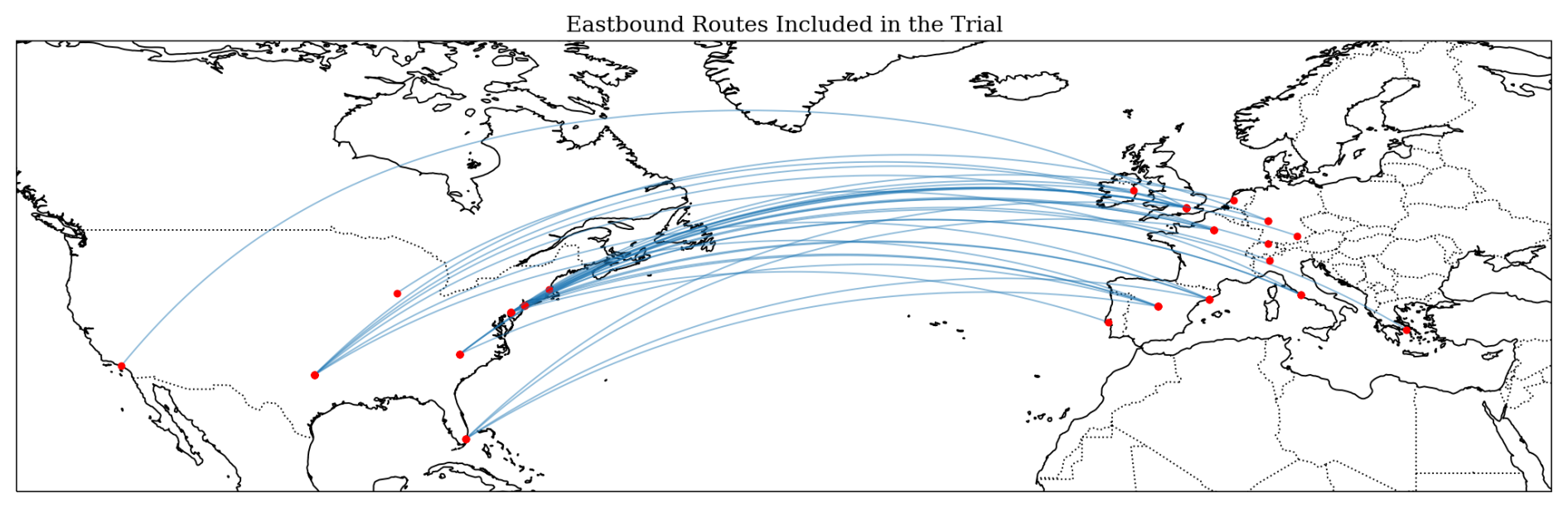
Figure 1Eastbound flight routes considered for this trial. The displayed routes are great circle paths between each city pair and do not necessarily reflect the actual paths that were flown. A full list of city pairs included in the trial and their applicable time periods is provided in Table C1.
2.2 Scope
For this trial, we considered all of AAL's eastbound flights from the United States to Europe, with certain flights removed from consideration due to operational constraints. All of the flights in the trial were part of AAL's standard schedule. The trial scope was explicitly defined as a set of origin-destination city pairs. Throughout the trial, 28 city pairs were considered, with certain city pairs added partway through the trial due to seasonal changes in AAL's flight schedule. Figure 1 shows a map of all city pairs considered for the trial. The eastbound flights to Europe primarily flew during the nighttime, meaning that any contrails produced by those flights were likely net warming. Therefore, this choice of scope also maximized the number of flights with high average contrail warming according to the forecast we used.
Every 2–3 weeks, each city pair was randomly assigned to the treatment or control group with a 50 % probability. The treatment/control structure of the trial will be discussed in detail in Sect. 2.4 and 2.7. The trial began with a “ramp-up” period, where city pairs were progressively added to the trial until week 5, when the trial included all candidate routes. A full list of city pairs and their applicable time periods is provided in Table C1.
The trial ran for 17 weeks beginning on 15 January 2025 and ending on 13 May 2025. The start and end dates were determined before the trial began and did not change depending on how many contrail avoidance flights were flown.
2.3 Flightkeys Optimizer
The Flightkeys platform performs trajectory optimization using a gridded approach, leveraging established path-finding algorithms such as Dijkstra's and A* (Frias et al., 2025, 2024). In this work, we refer to plans generated by the Flightkeys optimizer that do not consider contrails as “non-avoidance” plans.
For this study, forecasted contrail costs were included as an additional term in the cost function of the optimizer. The optimizer uses a marginal cost index to determine how heavily to weight contrails in the cost function. For this trial, we used a marginal cost value of USD 50 t CO2e−1. The Flightkeys platform coarse-grains the native 0.25° contrail forecast resolution to 1° by taking the average value. This resolution was chosen to balance between accuracy and compute resource usage. Frias et al. (2025) contains a further discussion of this design choice. The platform receives hourly updates to the contrail forecast with a forecast range of 24 h. In this work, we refer to plans generated by the Flightkeys optimizer that consider contrails as “contrail-optimized” plans.
2.4 Flight Selection and Operational Workflow
The Flightkeys system generates one or more non-avoidance plans for every flight in AAL's environment beginning roughly 24 h before departure time. For every flight within scope of the trial, the forecasted EF (based on the forecast described in Sect. 2.1) of the non-avoidance plans was calculated. This process was repeated multiple times before departure. If the accumulated contrail impact across the flight path was less than 10 Mg CO2e (equivalent to 10 tonnes CO2e), the flight was not considered for the trial. The goal of this filter was to only suggest contrail avoidance when the original plan was forecasted to cause substantial contrail warming. The 10 Mg threshold was chosen by examining simulated plans for a set of 95 pre-trial flights. The authors of this work manually chose an appropriate value that filtered out flights where the optimizer did not find a plan with significant contrail benefit.
For flights in the control group that exceeded the 10 Mg threshold, operations proceeded as normal without considering contrails, meaning that dispatchers were only presented with non-avoidance plans. Neither dispatchers nor pilots had any indication that a flight was included in the control group. These flights were later used for analysis to establish a baseline against which the treatment group was compared.
In the treatment group, flights whose non-avoidance plan exceeded the 10 Mg threshold were re-optimized including the contrails cost term. The result of this procedure is a flight plan that minimizes a combination of contrail formation, fuel consumption, and other operational costs. Since the Flightkeys system is a cost-based system, the contrail-optimized plan may not avoid all forecasted contrails, if for example the extra fuel cost incurred by performing the contrail avoidance is too large.
In AAL's operations, dispatchers exercise joint operational control with pilots and are responsible for planning flights and working with the pilots to ensure safe operations for the duration of the flight. Once the contrail-optimized plan was generated, dispatchers were presented with a single contrail-optimized plan and one or more non-avoidance plans for consideration. Having multiple candidate flight plans available is a standard workflow for dispatchers. Additionally, flights whose non-avoidance plan passed the 10 Mg threshold were indicated by a colored border in the Flightkeys user interface (UI), providing a visual cue for dispatchers to consider contrails for that flight. Dispatcher participation in the trial was voluntary, so the dispatcher for a given flight could decide to evaluate and release the contrail-optimized plan to the pilots or proceed as usual and evaluate and release a non-avoidance plan. If the dispatcher decided to release the contrail-optimized plan, the plan would be released with a tag indicating that contrails were considered for that flight and a remark informing the pilots that contrails were considered in the creation of the flight plan. Pilots were not provided any specific information about the location of contrail areas along or near the route.
2.5 Validation with Satellite Imagery
After the trial completed, we used a modified version of the “contrail to flight” attribution algorithm “CoAtSaC” (short for “Contrail Attribution Sample Consensus”) (Sarna et al., 2025), with modifications described in Appendix B, to determine whether an observable contrail was created by each flight. This automated system also calculates the number of attributed observable contrail kilometers for each flight, which we used as the primary metric for comparing the treatment and control groups. In this work, we refer to the results of this system as “observable contrail formation”.
The system takes input images from the GOES-East geostationary satellite's ABI (Goodman et al., 2019), and identifies contrails in those images using a machine learning computer vision algorithm (Ng et al., 2023). The next step is to obtain Automatic Dependent Surveillance-Broadcast (ADS-B) flight path data. The data was a combination of terrestrial and satellite ADS-B data licensed from FlightAware LLC and Aireon LLC respectively. We process the ADS-B data using the process described in Sarna et al. (2025). The system then attributes each flight to contrails by simulating the advection of the flight path using wind data from ECMWF ERA5 reanalysis (Hersbach et al., 2020). It then compares the advected flight tracks to the detected contrails and determines that the flight matches an observed contrail if they are close enough, according to thresholds determined in Sarna et al. (2025), with the difference that in this work we also considered whether the contrail and flights had similar altitudes (Appendix B). The algorithm considers all spatiotemporally nearby flights for attribution, not only the flights included in the trial.
The performance of the attribution system is discussed in depth in prior work (Sarna et al., 2025; Geraedts et al., 2026). In this work we are measuring the end-to-end performance of our forecast system, the optimizer, and the validation system.
In order to keep the authors of this work blinded to the results, the satellite attribution was not performed until after the trial completed.
2.6 Contrail Warming Estimates
Contrail warming cannot be observed directly, so we consider warming results based on CoCiP simulations to evaluate the efficacy of the trial in reducing contrail warming. A significant weakness in using such simulations to estimate the warming of individual flights is the difficulty in accurately predicting specific humidity (Gierens et al., 2020; Agarwal et al., 2022). In this work this difficulty is reduced, because we have actually observed the flights making contrails; therefore, the observations give us information about the humidity. When estimating forcing, we assign zero forcing to flights which are not observed making contrails, and a nonzero forcing to those observed making contrails. We use two methods for estimating the energy forcing for the flights which make contrails based on observations.
The “averaged forcing” method assumes that the avoided contrails are “average” contrails, with the properties of the average contrail based only on time of day, season and latitude, as given in Platt et al. (2024). Roughly speaking, this leads to contrails at nighttime being assigned a warming of ∼500 MJ m−1 while daytime contrails are assigned around 0 MJ m−1. In this work, we refer to this forcing estimate masked by observations as “observation-informed average forcing”.
Another method is to use the forecast weather. We use the IFS ensemble forecast, and we leverage the fact that we observed a contrail by averaging the CoCiP EF of only the ensembles which predict a persistent contrail. In the (rare) case where we observe a contrail but no ensemble member predicts a persistent contrail, we still want to assign a nonzero warming value. Therefore, we also include in the average the averaged forcing estimate, to ensure that a nonzero forcing is assigned to all observed contrails. This follows a similar procedure to Platt et al. (2024) for estimating contrail impact assuming contrail formation. In this work, we refer to this warming estimate masked by observations as “observation-informed ensemble forcing”.
2.7 Randomized Controlled Trial
From the treatment group determined by random city pair assignment and 10 Mg warming threshold above, we considered three subgroups for analysis. These subgroups were defined before any members of the team were unblinded to the satellite results.
-
Level 1 (L1). Entire treatment group
-
Level 2 (L2). Flights that were released as contrail-optimized plans (subset of L1)
-
Level 3 (L3). Flights that were released as contrail-optimized plans and flown as planned (subset of L2)
The Level 1 group represents the full intent-to-treat group. The Level 2 and 3 groups are per-protocol groups, meaning flights which adhered to the intervention we proposed, with differently strict definitions of protocol adherence (McCoy, 2017). The Level 2 group is the subset of the L1 group where the dispatcher released the contrail-optimized plan to the flight crew, meaning that the dispatcher voluntarily selected the contrail-optimized plan. Because operational circumstances sometimes result in the dispatcher releasing revised flight plans, in order to determine which plan was released to the flight crew we considered the last released plan before takeoff. The ratio of L2 to L1 flights (hereafter called the L2 L1 take rate, where “take rate” indicates the voluntary dispatcher engagement with contrail avoidance) was 15.4 %. The Level 3 group is the subset of the L2 group where the flight adhered to the released flight plan. We considered a flight to have adhered to the contrail-optimized plan if the difference between the planned warming per flight km and the flown warming per flight km was less than 0.001 Mg CO2e km−1, where the warming was computed using the same forecast as described in Sect. 2.1. This threshold roughly corresponds to a 5 Mg CO2e warming threshold for a 5000 km flight, which is the approximate length of many of the flights in the trial. This heuristic was determined before unblinding to the satellite results and was found to compare well with subjective human assessments of adherence performed by the authors of this work. These subjective assessments were performed by visualizing flight plans interpolated to the contrail forecast in the vertical, lateral, and time dimensions, and judging whether the flown ADS-B path matched the planned path. Examples of these visualizations are provided in Appendix D. This heuristic has the advantage of disregarding any non-adherence that was not near a contrail region. For example, if the flight climbed to its cruising altitude later than planned, but there were no contrail regions nearby, it could still be included in the L3 group assuming it performed the planned contrail avoidance maneuvers. The ratio of L3 to L1 flights (L3 L1 take rate) was 7.8 %.
The reduction in contrail formation in the L1 group represents the average contrail reduction achieved over all the flights in the trial. However, it is strongly influenced by the relatively low take rate, which is in turn influenced by the design of this specific trial and may not be broadly applicable to other contrail avoidance efforts. The L2 group represents the contrail reduction achieved when dispatchers select and release a contrail avoidance flight plan. The L3 group represents the contrail reduction achieved when contrail avoidance routes were flown.
Each of these three treatment groups were evaluated against the control group using the observed per-flight contrail kilometers (normalized by flight distance) as the primary trial endpoint.
2.8 Statistical Analysis
To compare contrail formation in the treatment and control groups, we computed the ratio of total observed contrail kilometers (computed as the length of the flight that is attributed to the observed contrails) normalized by total flight kilometers, referred to hereafter as the Observed Contrail Rate ():
where i are the flights in either group k (and k is one of treatment or control), Ci represents the contrail distance in kilometers, and Li represents the flight distance for flight i in kilometers. When computing Li, we used only the flight distance west of 30° W longitude where the contrail forecast was available and where contrails could be observed by the GOES-East satellite.
To compare the fuel consumption between the treatment and control groups, we computed the Fuel Rate similarly to the Observed Contrail Rate (Eq. 1):
where Fi represents the fuel usage per flight and Li the total length of the flight (not restricted to west of 30° W). Fuel usage data is actual data provided by AAL. The quantity used for this analysis is the actual fuel used while the aircraft is in the air, derived by subtracting the fuel weight when the aircraft touches down from the fuel weight when the aircraft leaves the ground. This does not include the fuel used during the taxi phases before takeoff and after landing.
Due to operational constraints, city pairs were only randomized every 2–3 weeks. This caused an imbalance of aircraft type between treatment and control groups. For example, 74 % of the control group flights were Boeing 777s, whereas only 50 % of the treatment group flights were 777s. See Fig. E1 for the aircraft type distribution across groups.
The physical properties of a contrail are dependent on the combination of aircraft and engine type involved in contrail formation (Jeßberger et al., 2013; Unterstrasser and Görsch, 2014). However, the effect of these differences on geostationary-observable contrail formation is an area of active research (Driver et al., 2025; Gryspeerdt et al., 2024). Additionally, fuel consumption differs by aircraft type. Therefore, we treated aircraft type as a confounder for both contrail distance and fuel and adjusted the statistical tests accordingly. We report both marginal and adjusted results. To adjust the test statistic by aircraft type, we first computed the Observed Contrail and Fuel Rates per aircraft type. We then computed the weighted mean for treatment and control groups using the same weights, which are derived from the aircraft prevalence in the total study population. We computed the difference in both Observed Contrail and Fuel Rates: λ(control)−λ(treatment) as our test statistics. Statistical significance was assessed using a non-parametric stratified permutation test with 10,000 permutations (Pesarin and Salmaso, 1993; Holt and Sullivan, 2023). To generate the null distribution, treatment labels were randomly shuffled among flights strictly within their respective aircraft type, preserving the aircraft-type confounding structure. A p value was computed as the proportion of permuted statistics exceeding the observed reduction. For observed contrail formation, we used a one-sided p value, and for fuel consumption we used a two-sided p value.
To estimate the confidence interval, we performed a stratified bootstrap analysis with 10 000 bootstrap samples. We created new sample datasets by randomly drawing flights with replacement from the original treatment and control groups, doing so strictly within their respective aircraft strata to maintain the study's balance. For each iteration, we re-applied the aircraft prevalence weights and computed a new test statistic. The 95 % confidence interval was derived from the 2.5 and 97.5 percentiles these 10 000 simulated statistics.
2.9 Counterfactual Analysis
The L3 observable results in this work are the best estimate of how much reduction in contrail formation can be achieved with the methods used in this work when contrail-optimized routes are flown. The methods above compare the L2 and L3 groups to the control group. One drawback of the L2 and L3 analysis is that there might be some correlation between contrail formation and what causes a flight to be selected for the L2 and L3 groups. For example, in interviews conducted after the trial completed, dispatchers mentioned that the take rate depended on how busy they were. One factor that might make the dispatchers busy is more demanding weather conditions such as storms or turbulence, which could also be correlated with contrail formation. It may also be more difficult for the Flightkeys optimizer to offer a flyable contrail-optimized plan when a flight has to avoid large contrail-forming regions. In order to address these potential issues, we additionally performed a counterfactual analysis to confirm that the reduction in observed contrail km between the L2 and L3 groups is due to contrail avoidance. If the reduction factors from this counterfactual analysis were significantly smaller than the reduction factors in the observed results, we would have suspected that some amount of the observed reduction resulted from factors other than our intervention.
At many points in the flight planning process, the Flightkeys system generated both contrail-optimized and non-avoidance plans for a given flight. For flights where the contrail-optimized plan was released, we performed the additional counterfactual analysis to isolate the effect of our intervention without any additional confounders. To do this, we chose one of the non-avoidance plans as a counterfactual for the actual plan. In order to determine which non-avoidance plan to use as a counterfactual for the flight, we examined multiple choices of non-avoidance plan and compared them against the flown path for flights that did not perform contrail avoidance (specifically, flights from the treatment group that were not part of the L2 set, “L1 not L2”). The choices we evaluated were the minimum cost plan and the most recent plan. To find the “minimum cost” plan, we examined all non-avoidance plans generated before the flight's departure and chose the plan with the minimum total cost as calculated by Flightkeys. The total cost is a combination of fuel and other costs such as delays and overflight charges (Frias et al., 2024). The results of that analysis are included in Sect. 3.4.
We used the choice of non-avoidance plan from that analysis to compute the differences in expected contrail distance between the counterfactual plan and the flown path, where expected contrail distance was computed using the ML formation probability forecast described in Sect. 2.1. Since the expected contrail distance is a forecast product, we also validated that the forecast agrees with observations to justify its use in this analysis.
We additionally performed a counterfactual analysis for the fuel usage. Lacking simulated fuel data for the flown path, we compared the simulated fuel value for the last-generated contrail-optimized plan to the non-avoidance plan computed nearest to it in time, whether preceding or following.
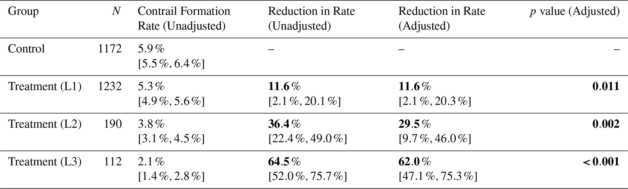
Table 1Observable contrail formation results for the control and treatment groups. Reduction in contrail formation rate is calculated with respect to the contrail formation rate in the control group. The “Adjusted” rate column incorporates the aircraft type adjustment described in Sect. 2.8, whereas the “Unadjusted” rate column does not. The values in brackets represent the 95 % confidence interval of the column quantity. Bold font in this table refers to the most critical results.
3.1 Observable Contrails
Table 1 shows the observed contrail formation rate for all the groups in our experiment. All subgroups of the treatment group showed a statistically significant reduction in observable contrail formation when compared against the control group. We rejected the null hypothesis of no change in observable contrail formation between the L1 treatment and control groups (one-sided p=0.011, stratified permutation test). We also rejected the null hypothesis of no change in observable contrail formation between the L2 treatment and control groups (one-sided p=0.002, stratified permutation test) and the L3 treatment and control groups (one-sided p<0.001, stratified permutation test). We see that the results are not substantially changed by the adjustment for aircraft type. Additional observed contrail values are included in Appendix F.
3.2 Contrail Warming Estimates
To estimate the warming reduction from our trial, we used the two methods described in Sect. 2.6. The results of the observation-informed average forcing analysis are shown in Table 2. We found significant reductions in all treatment subgroups. We rejected the null hypothesis of no change in observation-informed average forcing between the L1 treatment and control groups (one-sided p=0.006, stratified permutation test). We also rejected the null hypothesis of no change in observation-informed average forcing between the L2 treatment and control groups (one-sided p<0.001, stratified permutation test) L3 treatment and control groups (one-sided p<0.001, stratified permutation test).
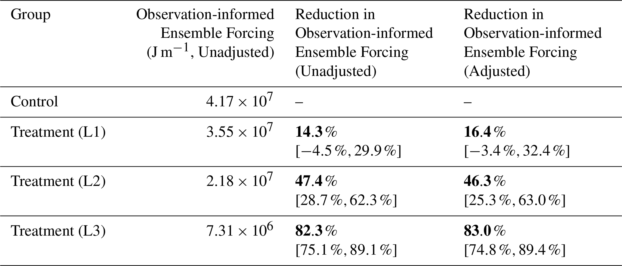
The results of the observation-informed ensemble forcing analysis are shown in Table 3. We rejected the null hypothesis of no change in observation-informed ensemble forcing between the L1 treatment and control groups (one-sided p=0.045, stratified permutation test). However, the confidence interval is relatively wide and crosses 0, indicating uncertainty in the warming reduction in the L1 group. We also rejected the null hypothesis of no change in observation-informed ensemble forcing between the L2 treatment and control groups (one-sided p<0.001, stratified permutation test) L3 treatment and control groups (one-sided p<0.001, stratified permutation test).
Table 2Observation-informed average forcing estimates for the control and 3 treatment group levels. Reduction in observation-informed average forcing is calculated with respect to the observation-informed average forcing in the control group. The values in brackets represent the 95 % confidence interval of the column quantity. Bold font in this table refers to the most critical results.
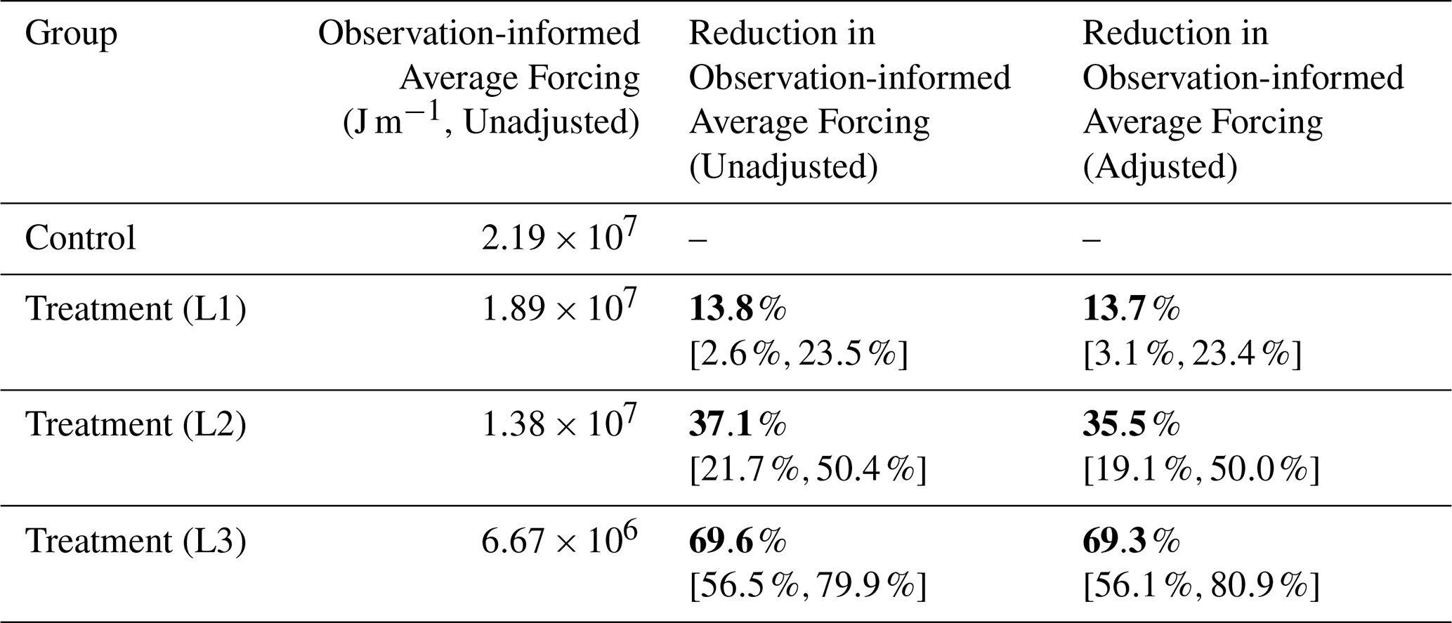
Table 3Observation-informed ensemble forcing estimates for the control and 3 treatment group levels. Reduction in observation-informed ensemble forcing is calculated with respect to the observation-informed ensemble forcing in the control group. The values in brackets represent the 95 % confidence interval of the column quantity. Bold font in this table refers to the most critical results.
3.3 Fuel Usage
Contrail avoidance may incur additional costs, both monetary and climatological, primarily in fuel usage (Teoh et al., 2020; Frias et al., 2024; Dean et al., 2025). This extra fuel is critical to quantify due to the climate impact from burning extra fuel. As previously noted, the Flightkeys optimizer used for generating contrail routes considers multiple costs, including fuel, contrails (with the specific price assignment for this trial), and others such as delays and overflight charges (Frias et al., 2024).
Table 4Fuel usage for the three treatment group levels. Differences in fuel usage are calculated with respect to the fuel usage in the control group. The “Adjusted” usage column incorporates the aircraft type adjustment described in Sect. 2.8, whereas the “Unadjusted” usage column does not. Negative differences indicate that the treatment group used less fuel than the control group, and positive differences indicate that the treatment group used more fuel. Bold font in this table refers to the most critical results.
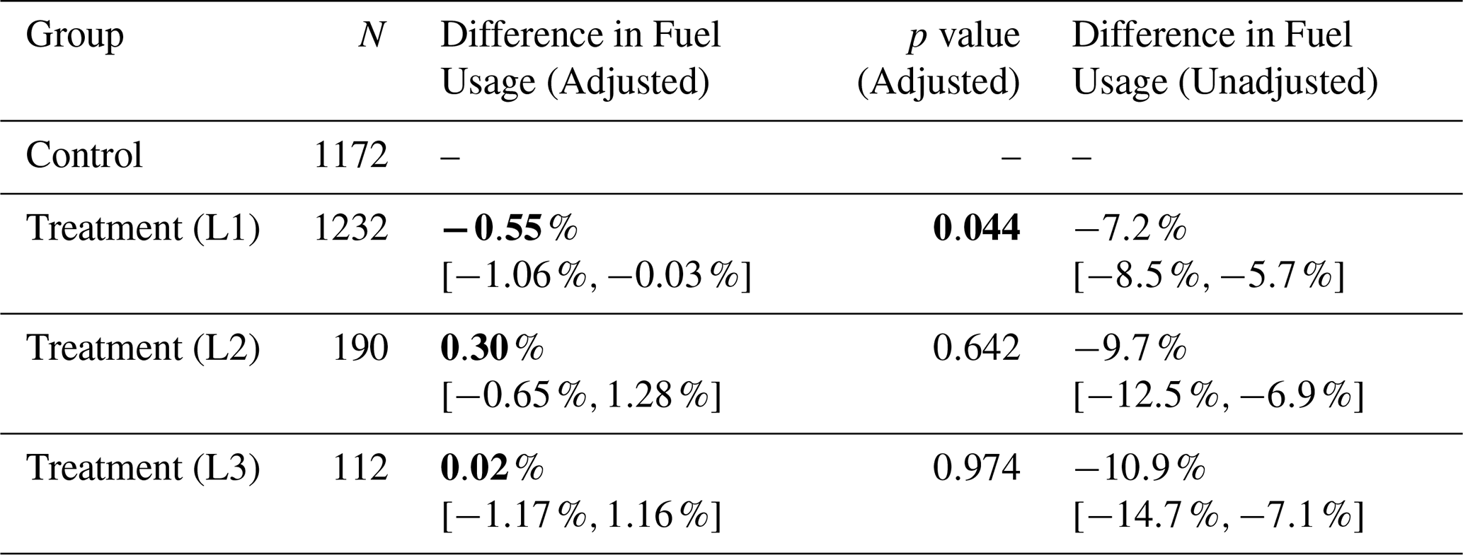
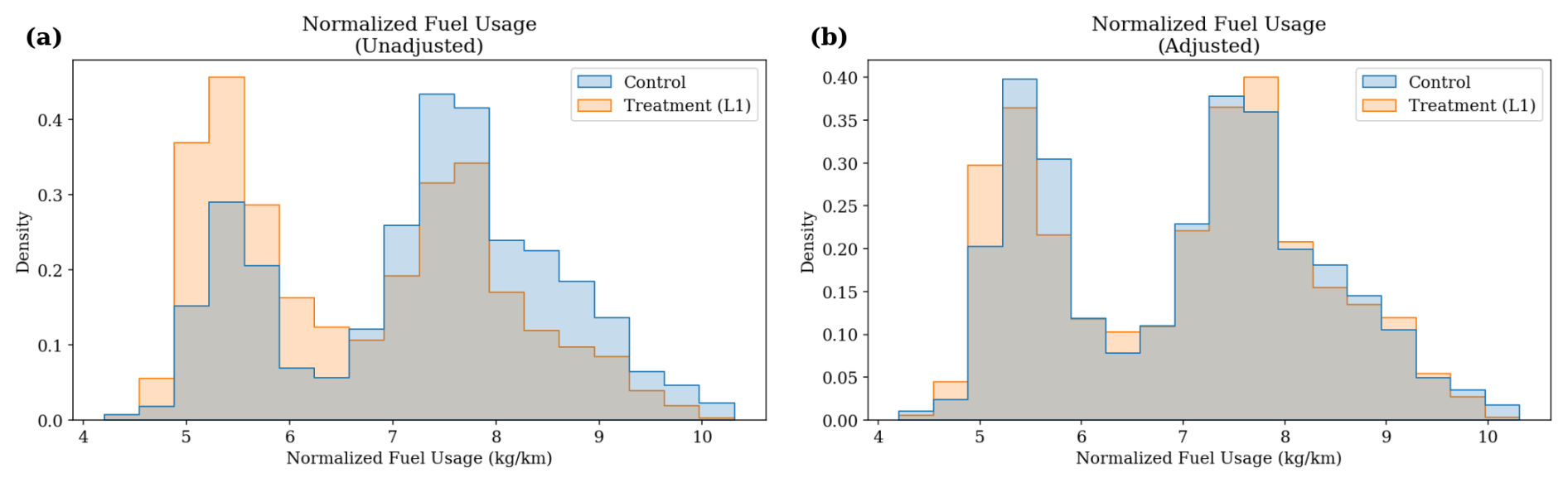
Figure 2Histogram of fuel/flight distance for each flight in the control and treatment groups. Two peaks correspond to the two different aircraft types in the trial: Boeing 777 and Boeing 787. In panel (a), the groups have different flight counts per peak; this imbalance is mostly removed in panel (b) after adjusting for aircraft type.
Using actual fuel data provided by AAL, we compared the fuel usage between the control group and treatment subgroups. The results from this analysis are shown in Table 4. The unadjusted numbers show a large reduction in fuel in the treatment group. The flights in the trial included two aircraft types: Boeing 777 and Boeing 787. Figure 2 visualizes the distribution of fuel per flight distance for each flight, demonstrating the aircraft type imbalance and effects of the adjustment described in Sect. 2.8.
Even after the aircraft type adjustment, we were able to reject the null hypothesis of no change in fuel usage between the L1 treatment and control groups with relatively high confidence (two-sided p=0.044, stratified permutation test). However, the difference is small (<1 %) and the test is close to not being statistically significant at the p=0.05 level. The remaining difference may be due to other residual confounders such as different city pairs having slightly different average fuel usage, differences in weather, or differences in load factor. We are unable to reject the null hypothesis of no change in fuel usage between the L2 treatment and control groups (two-sided p=0.642, stratified permutation test) and the L3 treatment and control groups (two-sided p=0.974, stratified permutation test).
3.4 Counterfactual Flightkeys-Generated Plans
In the previous section we found a small reduction in fuel usage in the treatment flights which implemented contrail avoidance. We suspect that this difference is due to uncontrolled confounders such as different weather patterns between treatment group days and control group days. In this section we study whether these confounders could also be responsible for the observed differences in contrail formation between the treatment and control groups.
To do this, we compare the contrail avoidance plans in the treatment group to the non-avoidance plans on the same flights, which we call the “counterfactual” plans.
The advantage of doing this counterfactual analysis is that since the flights are the same, confounders such as city pair and weather cannot be responsible for an observed reduction. Figure 3 shows the results of the analysis described in Sect. 2.9 to select which non-avoidance plan to use as a counterfactual. Since the “minimum cost” plan compares best against the flown values, we use this plan for subsequent analysis.
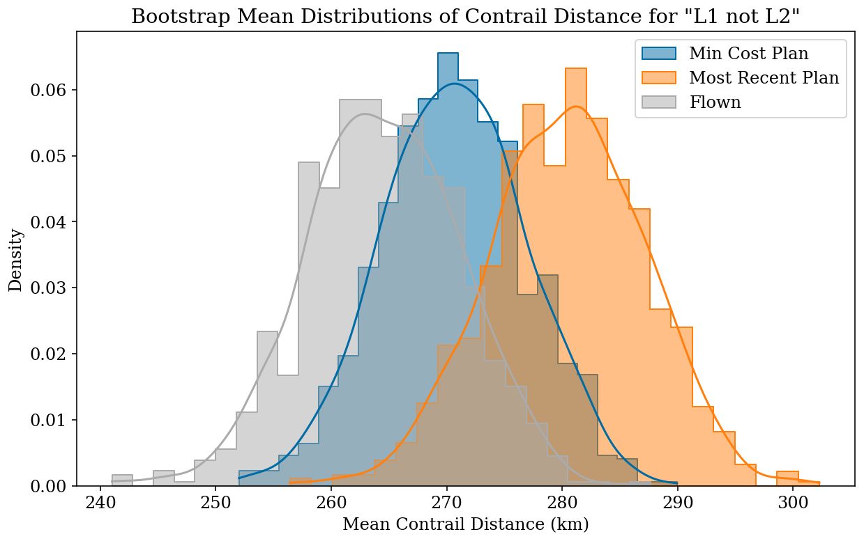
Figure 3Bootstrap mean distributions of expected contrail distance for two potential choices of counterfactual plan (minimum cost plan and most recent plan before takeoff) compared against the flown path for flights in the L1 group where the contrail avoidance plan was not released (“L1 not L2” flights). The minimum cost counterfactual plan matches better to the flown values.
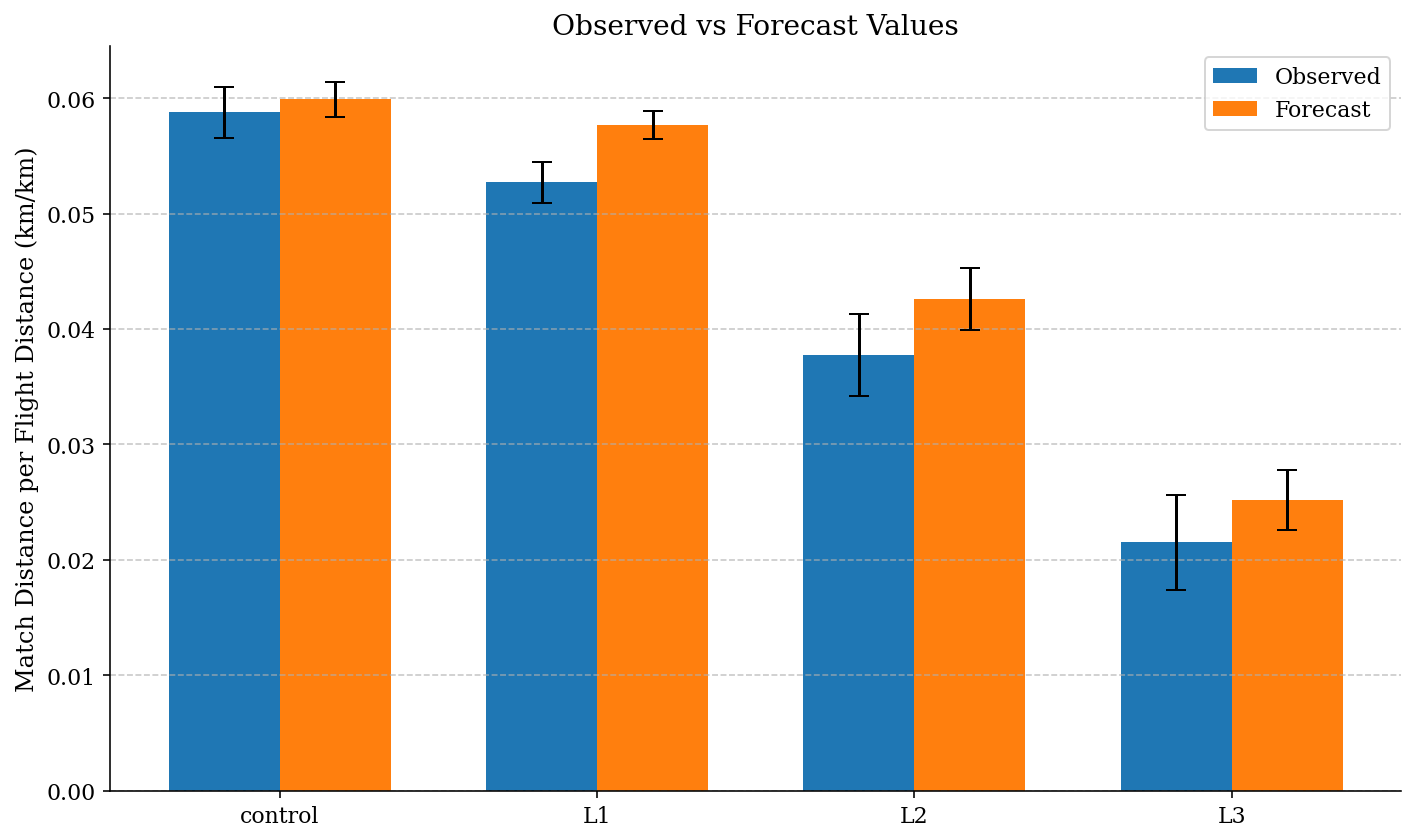
Figure 4Comparison of the ML formation probability forecast vs. observed match distance per flight distance for the control and 3 treatment groups in the trial. The value of the bar is the mean match distance per flight distance for the group, with error bars showing the standard deviation. For each group, the forecast agrees with the observations.
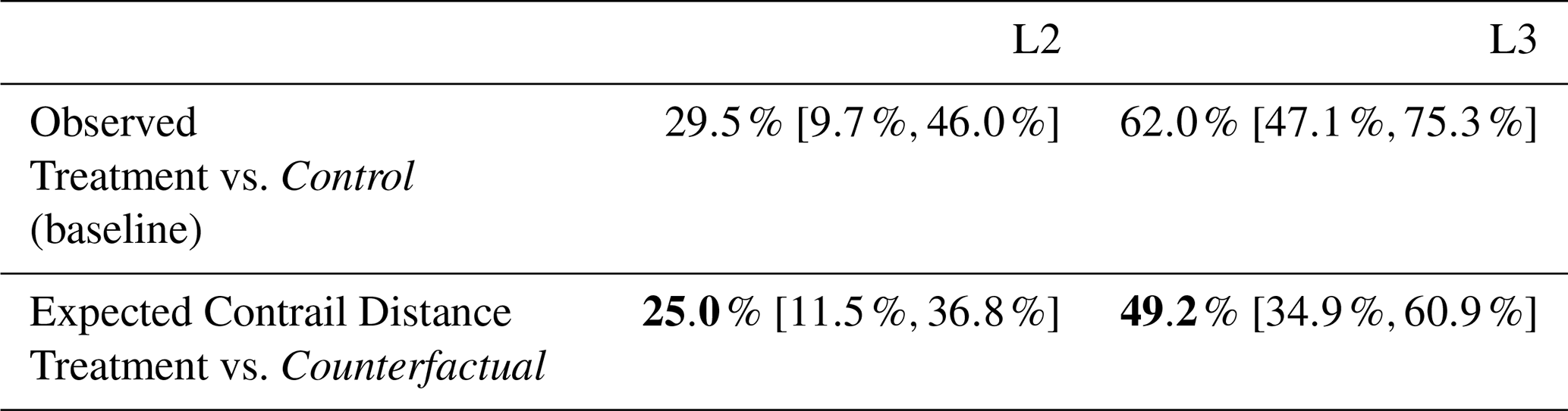
Table 5Contrail distance reduction factors of the two per-protocol groups evaluated against the counterfactual plans. Expected contrail distance uses the counterfactual plan. Observed results are reproduced here from Table 1 as a baseline. The values in brackets represent the 95 % confidence interval of the column quantity. Bold numbers indicate that those are the primary results of the table. Italic font here is meant to draw attention to the fact that the point of comparison in the two rows of the table are different.
A drawback of the conterfactual method is that since the counterfactual plan was not flown, we cannot use observations for this analysis. Instead, we evaluate the expected contrail distance from the contrail forecast. As discussed in Sect. 2.1, the final forecast output is the product of an ML-predicted contrail formation probability and an averaged forcing estimate. However, in the analysis shown in Sect. 5 we report on the contrail length reductions because they are more easily directly observable. The contrail probability may not in general agree with observations on an individual flight, since the probability ranges from 0–1 while the observation-derived label from the CoAtSaC algorithm is either 0 (no contrail observed) or 1 (contrail observed). However, over a large number of flights these differences average out. As shown in Fig. 4, the ML contrail forecast probability agrees with observations when aggregated over our treatment and control groups, justifying its use as a proxy for the observed results.
The results of this analysis are shown in Table 5. We see that when evaluated against the counterfactual plan, the reduction factors are smaller than the reductions seen in the observed results. However, the error bars between the counterfactual reductions and the observed reductions overlap significantly, and both treatment vs. counterfactual comparisons achieved statistical significance when evaluated using the permutation test (p<0.001). Note that we do not use the stratified permutation test here since the counterfactual and treatment groups will have the same aircraft type distributions by construction. This counterfactual analysis demonstrates that the observed difference between the treatment and control groups cannot be explained by confounding differences in the flights chosen for each group.
In order to perform a similar analysis for fuel, we selected the most recently created contrail-optimized plan as the “treatment flight plan” and the non-avoidance plan that was created closest in time to the treatment flight plan to be the “control flight plan”. Similarly to the observed results, the simulated fuel comparisons do not achieve statistical significance for the L2 and L3 groups (L2 p=0.855, L3 p=0.868, permutation test).
This study describes a scalable large-scale Randomized Controlled Trial that demonstrates the feasibility and efficacy of navigational contrail avoidance within a commercial airline's standard operational workflow. By integrating contrail forecasts directly into the Flightkeys flight planning software, we enabled dispatchers to execute avoidance maneuvers without the need for bespoke communication channels. The results provide strong evidence that navigational contrail avoidance is effective in reducing observable contrail formation and operationally feasible in realistic circumstances.
In the intent-to-treat group (Level 1, n=1232), we observed an 11.6 % [2.1 %,20.3 %] reduction in observable contrail formation relative to the control group. This value is statistically significant (p=0.011), though the uncertainty of the overall size of the effect is large. Based on these observations, we estimated the warming reduction to be 13.7 % [3.1 %,23.4 %] with the observation-informed average forcing method (p=0.006) and 14.3 % (p=0.045) with the observation-informed ensemble forcing method.
These figures represent the aggregate benefit across the entire network subset, including flights where no action was taken. The efficacy of the intervention becomes most apparent in the per-protocol analysis (Level 3, n=112), which isolates flights that successfully flew the contrail-optimized plans. In this group, observable contrail length was reduced (p<0.001) by 62.0 % [47.1 %,75.3 %], observation-informed average forcing was reduced (p<0.001) by 69.3 % [56.1 %,80.9 %], and observation-informed average forcing was reduced (p<0.001) by 83.0 % [74.8 %,89.4 %]. This substantial gap between the intent-to-treat and per-protocol results highlights that while the physical mechanism of avoidance is highly effective, the operational execution – specifically the “take rate” of the plans – remains a primary bottleneck for network-wide scaling.
By utilizing the CoAtSaC automated contrail-to-flight attribution algorithm (Sarna et al., 2025), we were able to objectively validate performance across thousands of flights using GOES-East imagery. This methodology establishes a new standard for validating the efficacy of contrail avoidance trials, proving that contrail reductions can be quantified using peer-reviewed methodologies at large scales.
In this work we are reporting a 62.0 % reduction in contrails observable via geostationary satellite, but not all contrails are observable. In particular, the GOES ABI images have a nadir resolution of 2 km, which makes it difficult to detect young, narrow contrails. The reductions in total contrail distance and contrail warming are likely smaller if one assumes that some unobservable contrails are less affected by the contrail avoidance performed in this test. What fraction of contrails (and contrail warming) are observable is a subject of active research. For example, Euchenhofer et al. (2025) compared a set of GOES ABI images to higher-resolution low-Earth orbit (LEO) satellite images and found that 42 % of the higher-resolution contrail distance was visible in the nearest GOES scan. However, we should note that the CoAtSaC algorithm (Sarna et al., 2025) only requires detecting the contrail in at least two scans captured during its lifespan, so having some frames where it is detectable in LEO but not in GOES is not inherently problematic. Furthermore, since more warming contrails tend to be larger with higher optical depth, they are also generally easier to detect in a GOES-ABI image, so the fraction of warming that is observable may be larger than the fraction of contrail distance. For example, Driver et al. (2025) used radiative transfer simulations to estimate that, in the clear sky case, 45 % of contrail distance is observable in a given GOES ABI frame, but 57 % of contrail distance and 97 % of contrail long-wave energy forcing comes from contrails observable at some point in their lifetime. Further research is needed to better quantify the fraction of contrail warming that is observable.
Operational integration presented specific challenges that influenced the trial's outcomes. The “take rates” of 15.4 % (flights released as contrail plans vs. total candidate flights) and 7.8 % (flights released as contrail plans and flown as planned vs. total candidate flights) are relatively low. Given the complexity of even routine daily aircraft operations, there are a large number of reasons why a contrail plan might not be released, or a released plan might not be flown. In interviews with participating dispatchers, a few common cases were discussed and summarized here as follows. Dispatchers found that contrail avoidance plans sometimes involved descents and ascents in the middle of a flight, which are safe and done in coordination with air traffic control, but which the dispatchers and flight crews preferred not to do. In the North America to Europe flights included in this trial, AAL preferred to adhere to the North Atlantic Organised Track System (OTS), and Flightkeys had special user interface features to make this easy for the dispatchers. These features were for technical reasons not able to be activated for the contrail flights during this trial, making contrail avoidance more difficult near the OTS tracks, which in many cases led to dispatchers choosing not to attempt contrail avoidance on those flights. Due to such issues, the take rate of dispatchers releasing a contrail-aware flight plan ranged widely per city pair. Dispatchers also mentioned that their take rate was typically lower when they and the aircraft crew were busier. As this trial was executed on a voluntary basis, a dispatcher could also choose to not take part for any reason. Dispatcher priorities were established with safety as the primary focus, followed by efficiency and finally contrails. The L2 L1 take rate on a per-dispatcher basis ranged widely, suggesting that inter-dispatcher variation is important. Since city pairs were not evenly distributed between dispatchers, this likely had an effect on the difference in take rate per city pair. Finally, dispatchers mentioned the presence of turbulence, which is a safety concern, as a reason for not considering the contrail-optimized flight plan. Further research is necessary to understand the correlation between turbulence and contrail formation.
A few software improvements could improve the take rate for future trials. In the user interface available to dispatchers for this trial, there was only a top-down view of the contrail avoidance regions, but additionally including a vertical profile view would be beneficial. This made it difficult for dispatchers to understand why certain adjustments were happening.
Improvements to the user interface inside flight planning software could lead to a larger observed contrail reduction, even in the L3 group. Dispatchers frequently make manual adjustments to software-optimized plans, even when contrails are not considered. In a few (2–3) instances in the trial, dispatchers, without the benefit of the vertical profile view of the contrail avoidance regions, adjusted a contrail-optimized plan to fly through the contrail avoidance region, but these flights nonetheless ended up in the L3 group.
Around half of the released contrail-optimized flight plans were not flown as planned, as determined by the L3 criteria. This could potentially be ameliorated by displaying contrail information in tools accessible to pilots such as the “Electronic Flight Bag” (EFB), so that pilots can also understand why maneuvers are being made. Additionally, the automated flight planning process starts roughly 24 h prior to departure, and the dispatchers engage with the process closer to the departure time. The contrail forecast can change during that time. If a flight was initially exceeding the 10 Mg threshold, a dispatcher could start working on a contrail plan even if later updates to the weather forecast brought the flight below the 10 Mg threshold. This could have also occurred in the control group and therefore should not substantially affect the results, but it might have caused flights whose non-avoidance plans had low contrail impact to end up in both the treatment and control groups. Future improvements to flight planning software could ameliorate both of these problems. Additionally, in a system-wide deployment of contrail avoidance, the efficacy of the contrail avoidance regime may improve since dispatchers would only be presented with flight plans that consider contrails, rather than being presented with multiple non-avoidance and contrail-optimized plans from which to choose.
Our analysis of fuel burn revealed a counter-intuitive result: the Level 1 treatment group appeared to consume 0.55 % less fuel than the control group (adjusted p=0.044). As detailed in Sect. 3.3, this finding is likely driven by residual confounding within the randomization structure rather than a genuine fuel benefit of contrail avoidance. This “negative cost” result, along with the ≈2 percentage-point-wide confidence intervals for fuel reduction in the L2/L3 groups, underscores the difficulty of isolating the fuel penalty of avoidance (estimated at 0.1 %–0.2 % across all of an airline's flights; Teoh et al., 2020; Frias et al., 2024; Dean et al., 2025) against the high variance of real-world fuel consumption data. Understanding the fuel penalty is critical for assessing the climate impact of contrail avoidance, since additional fuel usage is accompanied with higher emissions and climate impacts of CO2 and non-CO2 gases and aerosols. Larger sample sizes and stricter randomization protocols in future trials will be necessary to precisely quantify the fuel penalty trade-off.
Finally, while our counterfactual analysis suggests that the observed reductions were not driven by dispatchers selecting flights that would have formed fewer contrails even without our intervention, the infrequent randomization of city pairs remains a limitation. To further establish causality and refine the cost-benefit analysis, future work could expand beyond the North Atlantic to a global scope to ensure that the methods proposed here work in more congested airspace, increase the frequency of randomization, and further automate the optimization workflow to reduce labor burden on dispatchers. Future work should also explore different operational concepts for contrail avoidance such as coordination between airlines and Air Navigation Service Providers (ANSPs), ANSP-led trials, or coordination between multiple airlines. Despite these limitations, this trial provides a statistically robust point of evidence that commercial aviation can successfully avoid warming contrails using existing operational infrastructure.
NWP models and their reanalysis products are known to contain biases in atmospheric humidity fields when compared to observations (Agarwal et al., 2022; Gierens et al., 2020). In order to account for this uncertainty, we used a machine learning model to predict geostationary-observable contrail formation from NWP output fields, effectively acting as a debiasing operator against contrail observations on the NWP outputs. Similar approaches for ML debiasing of humidity have been discussed in the literature (Wang et al., 2025).
Model Construction
The ML model was trained using weather fields as inputs and contrail formation labels from the automated flight-to-contrail attribution algorithm described in Sarna et al. (2025) with the modifications from Appendix B. The training data for the model consisted of flight waypoints labeled by whether that flight waypoint formed a contrail.
Table A1Weather variables and summary statistics provided as input features to the ML forecast model. Variables in italics are only provided at the original flight waypoint and are not summarized using the summary statistics.
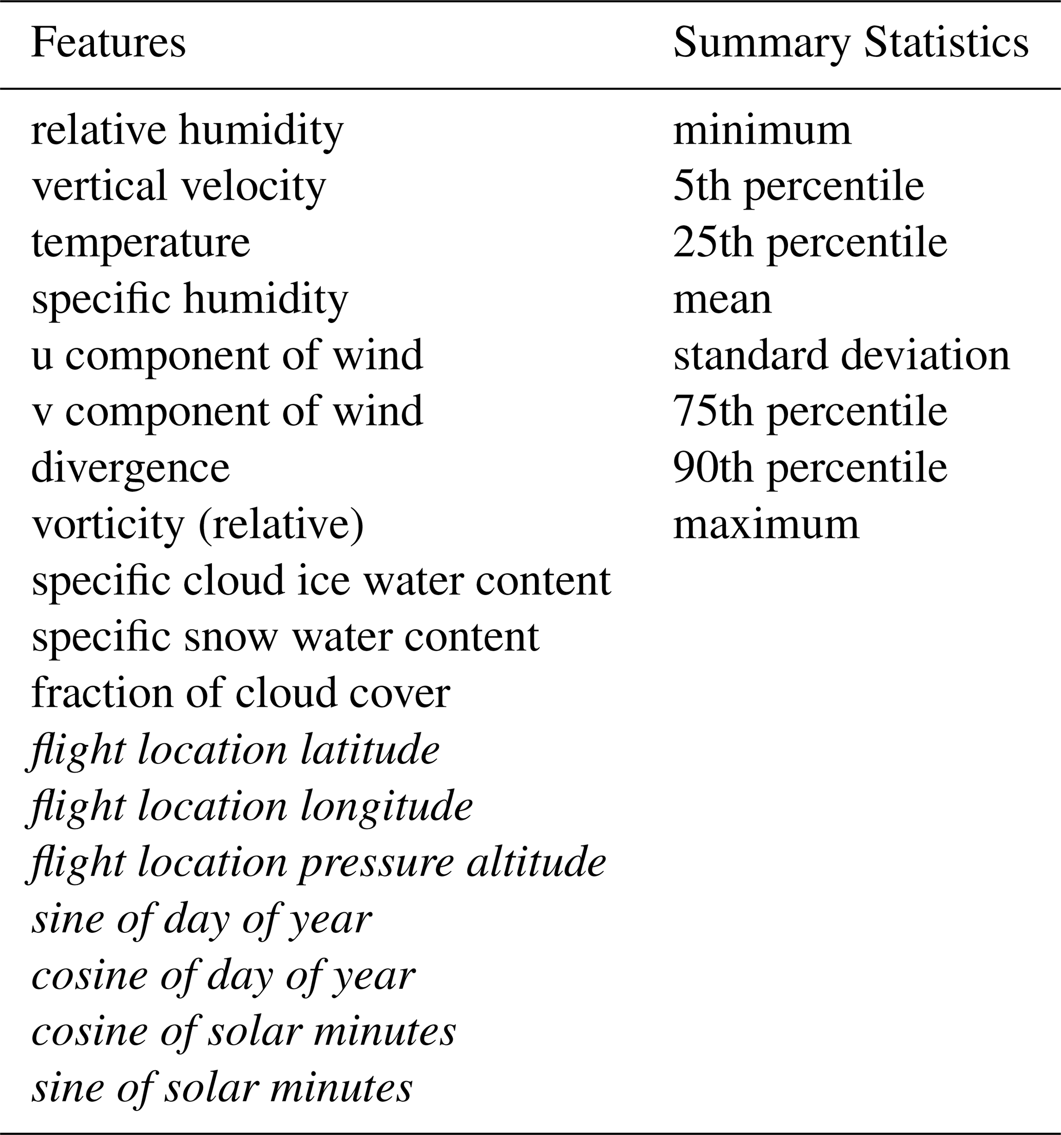
In order to create input features for the model, each flight waypoint was advected in 3 dimensions with the NWP output winds using the third-order Runge-Kutta method (Bogacki and Shampine, 1989) with 10 min timesteps for a total of 2 h. At each advected location, weather features were read from the NWP outputs. For each weather variable, its values across the advected path were summarized using a variety of statistics. These summary statistics were given to the ML model as input features. The model also received additional features about the flight location and time of day. A full list of input features and statistics is provided in Table A1.
The ML model is a 4-layer deep neural network, trained using the AdamW optimizer with cross-entropy loss. The hyperparameters of the model were optimized using a hyperparameter search. We additionally applied a calibration on the model outputs against a held-out set of the contrail formation labels to translate the model outputs into calibrated probabilities. More information about the ML forecast is available in Sonabend-W et al. (2024).
The performance of the ML contrail forecast model is evaluated in ContrailBench (Hodgson and Abbott, 2026). In the operational workflow described in this trial, the forecast is treated as a continuous value; therefore, multiple operating points on the ContrailBench curve will be relevant in practice.
During development, the model was constructed and validated using the freshest available NWP forecast weather. The model's performance at operational forecast lead times is not assessed directly, but prior work suggests that contrail forecasts are performant at operationally-relevant lead times (Dean et al., 2025). The trial described in this work is also designed to assess the forecast performance at operationally-relevant lead times.
For the validation system for the trial described in this paper, we used a modified version of the contrail-to-flight attribution algorithm described in Sarna et al. (2025). The modified version of this algorithm is also used for generating training data for the ML contrail formation forecast.
B1 Contrail Altitude Model
We developed a system to infer the altitude of a contrail in GOES imagery, similar to the method introduced in Meijer et al. (2024). The system uses a convolutional neural network (CNN) that takes radiances from tiles of the GOES imagery as input and infers an altitude at each pixel in the tile. This CNN is trained using altitudes from flight-to-contrail attributions as labels. Specifically, during the attribution process, the advection of exhaust plumes from flights are simulated in 3D space from their original locations to the times of satellite images, as described in Sarna et al. (2025). If the attribution algorithm finds a matched flight for a given detected contrail, the advected altitude of that flight is used as the label for the pixels spanned by the detected contrail. Detected contrails that do not have a matched flight are not included in the training data. The loss is only applied on pixels where the dataset includes a detected contrail with a corresponding matched flight.
In order to account for the effects of viewing angle on the perceived altitude by the satellite, we transform the advected barometric altitude of the flight into a “radiative path length”, which allows the altitude estimation model to take into account the amount of atmosphere through which the satellite-sensed radiation traveled between the earth surface and the observed contrail. To perform this transformation, we first interpolate the advected pressure level in ERA5 reanalysis data to find its corresponding geopotential height, and then convert that to geodetic height by dividing it by the acceleration due to Earth's gravity. We then apply trigonometric identities (visualized for a simplified 2D case in Fig. B1) to translate the geodetic height into a radiative path length. After the model performs inference, the inverse of this trigonometric transformation is used to translate the radiative path length back to a geodetic altitude.
During the training process, the model is validated against a held-out set of flight-to-contrail attributions. This dataset has the advantage of wide spatiotemporal coverage, but has the disadvantage of incorporating the noise introduced by the inaccuracies of the attribution algorithm. In order to ensure that the model performs well and generalizes, we additionally evaluate its performance on the LiDAR colocation dataset from Meijer et al. (2024) that provides high-accuracy altitude estimations from the CALIOP instrument onboard the CALIPSO satellite. On this dataset, our model achieves a root mean squared error (RMSE) of 789 m, compared to the RMSE of 570 m from Meijer et al. (2024). We chose not to use the CALIOP data for training data generation in the model since CALIPSO was decommissioned in 2023. Since the RMSE of this altitude estimation is greater than 2 flight levels (2000 ft = 609.6 m), we use it as a coarse filter in the modified attribution algorithm described below.
At inference time, the model produces an inferred altitude for every pixel in the input satellite image, regardless of whether there is a contrail present. In order to use these inference results in the downstream attribution algorithm, we join the inferred altitudes with detected contrails from Ng et al. (2023). Each linearized contrail is assigned the mean altitude of the inference results from the pixels it contains.
B2 Modified Contrail-to-Flight Attribution Algorithm
At a high level, the system described in Sarna et al. (2025) begins by considering attributions in each frame of the satellite imagery and looks for patterns in how those single-frame attributions evolve over time through multiple frames of the satellite image. The key modification we make to this algorithm is to filter out single-frame attributions where the advected altitude of the flight is significantly different from the inferred altitude of the detected contrail as determined by the CNN. We set the threshold as
where RMSEaltitude is the root-mean-squared error of the altitude model from the previous section (800 m) and RMSEadvection is the vertical root-mean-squared error introduced during advection due to imperfect wind data. RMSEadvection is computed independently of the advection age by comparing the advected altitude to the known synthetic altitude of contrails in SynthOpenContrails (Sarna et al., 2025), and is estimated at 111 m. Equation (B1) therefore evaluates to 1615 m. If in a single satellite frame the inferred contrail altitude differs from the advected flight altitude by more than 1615 m, the single-frame attribution is not considered as a candidate match for the subsequent multitemporal aspects of the algorithm. Since 1615 m is greater than 5 flight levels (5000 ft), this is a coarse filter which conservatively removes highly unlikely candidate flight-contrail matches; the algorithm does not require strict agreement between the advected flight altitude and inferred contrail altitude. In order to evaluate the effect of this modification on the performance on CoAtSaC, we designed a version of the evaluation of CoAtSaC against SynthOpenContrails that assumes an RMSE of the altitude estimator and assigns the synthetic predicted altitude of a contrail to a value sampled from a Gaussian where the mean is the known altitude of the contrail and the standard deviation is the RMSE of the altitude estimator. This synthetic predicted altitude is used in place of the inferred altitude of the detected contrail in the modified algorithm described above. With this change, the “flight precision” on the tracking subset of SynthOpenContrails improves from 71.4 % to 79.4 %.
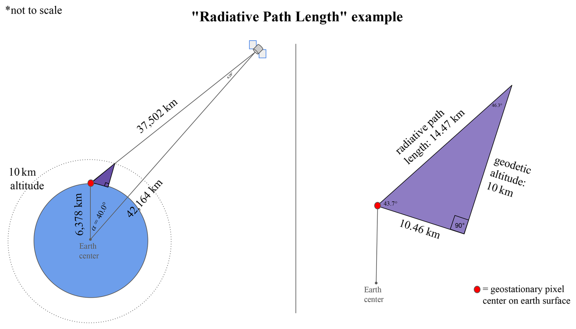
Figure B1Example of a transformation from geodetic altitude to radiative path length. This simplified example considers a contrail that is over the Equator at 40° longitude away from the nadir of the geostationary satellite. Its geodetic altitude is 10 km, which is translated into a radiative path length of 14.47 km using the triangle formed by the satellite, contrail, and center of the Earth and the purple triangle formed by the contrail, the point directly underneath it on the surface, and the point on the surface that the satellite is viewing for the pixel in which the contrail appears. Side lengths and angles other than the 40 degrees longitude, Earth radius, and geostationary orbit distance are derived via trigonometric identities.
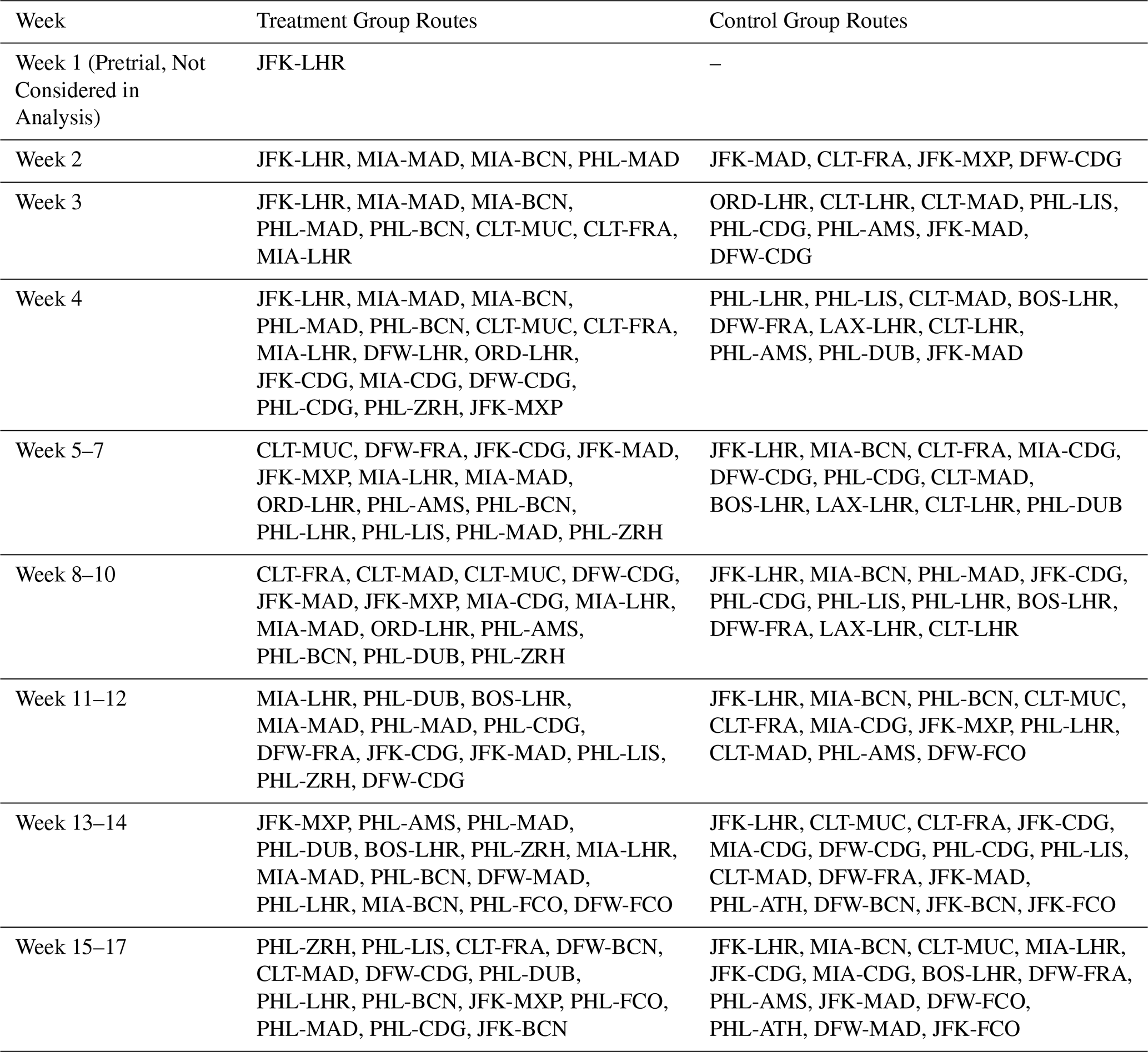
Table C1 shows the city pair assignments by week in the treatment and control groups.
Table C1Flight route assignments by week and group. Week 1 began on Wednesday, 15 January 2025. Each week of the trial started on Wednesday and ended on the following Tuesday.
Figures D1 and D2 show examples of the visualization used by the authors of this work to assess flight plan adherence.
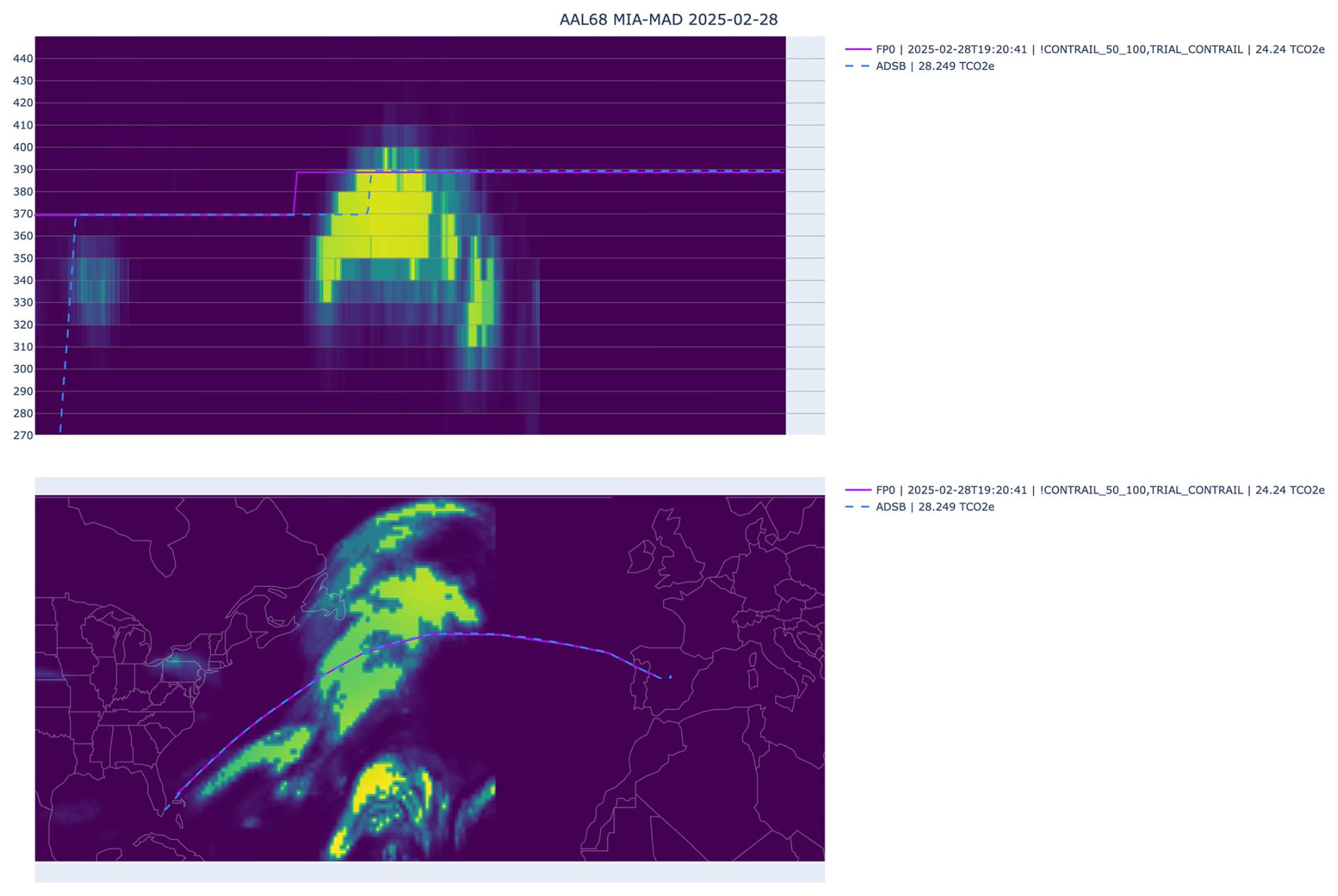
Figure D1Example of an L2 flight that is not included in the L3 set. Dashed blue lines represent the flown path, and solid purple lines represent the planned path. The top image shows the vertical altitude profile, where the green colors represent the contrail forecast interpolated to the flown path. The bottom image shows the lateral profile, with the contrail forecast at a fixed 35 000 ft.
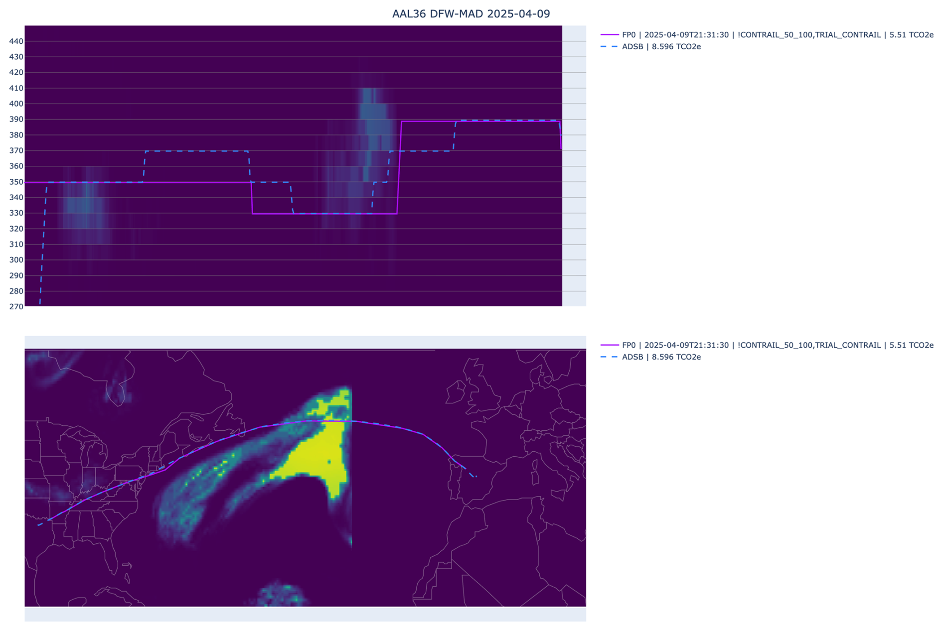
Figure D2Example of an L3 flight. Despite imperfect adherence to the vertical profile, the difference in forecasted contrail impact is not large enough to fail the L3 inclusion check. Dashed blue lines represent the flown path, and solid purple lines represent the planned path. The top image shows the vertical altitude profile, where the green colors represent the contrail forecast interpolated to the flown path. The bottom image shows the lateral profile, with the contrail forecast at a fixed 35 000 ft.
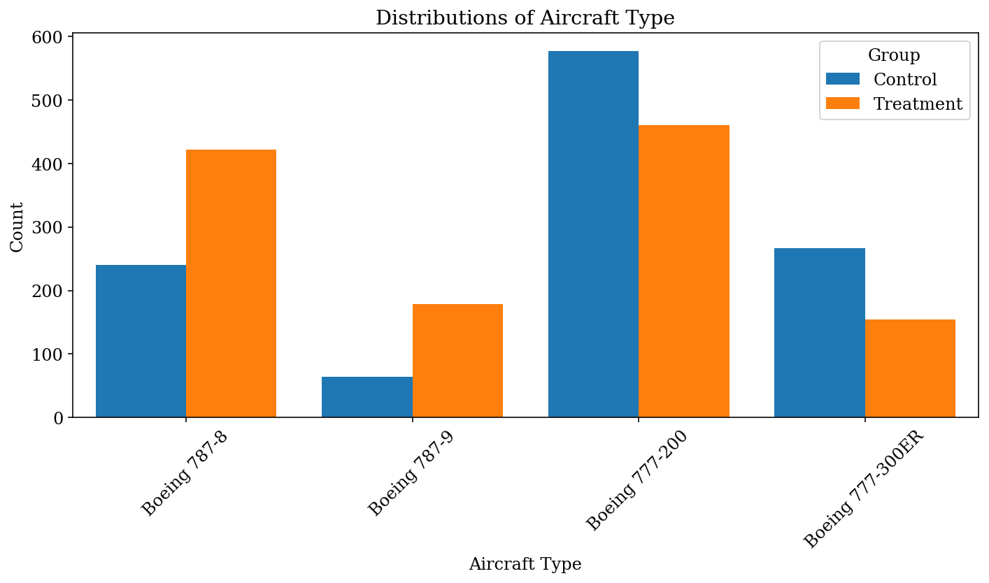
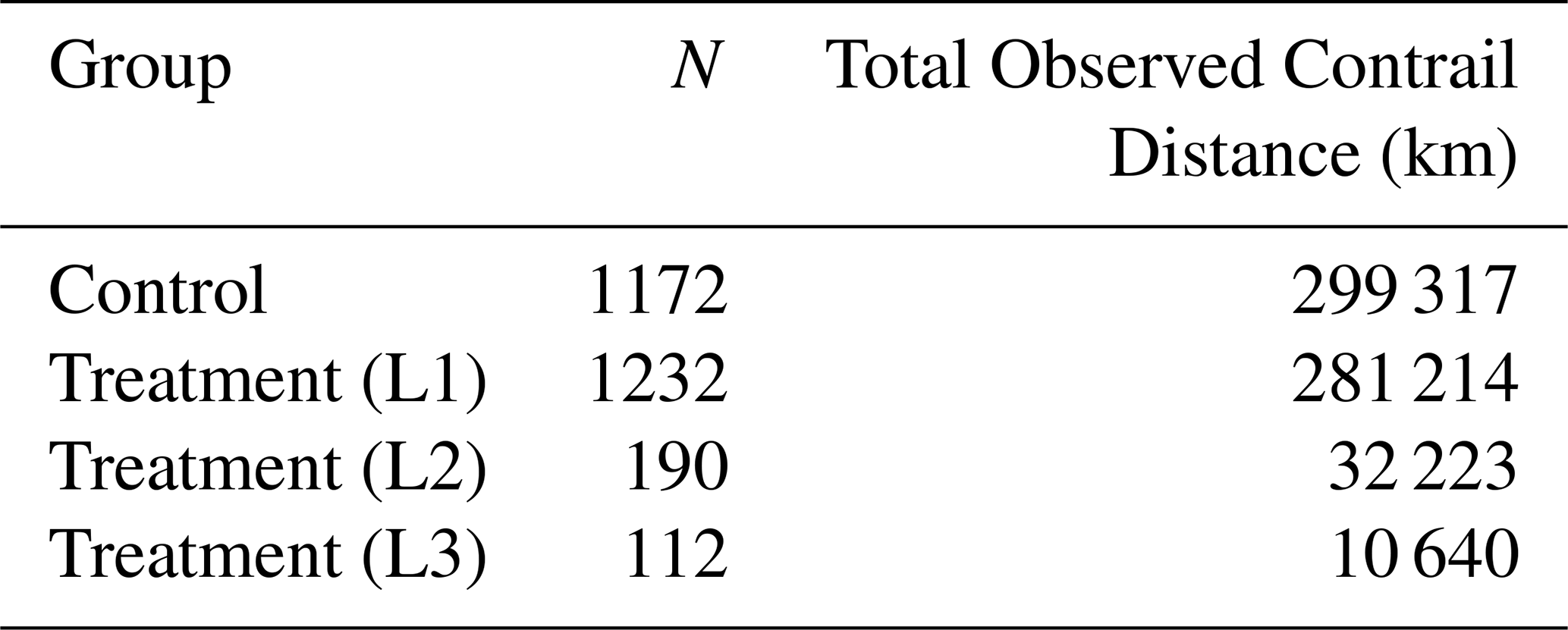
Table F1 shows additional observed contrail values.
Table F1Observed contrail formation results and total observed distances.
The accompanying dataset and code for this paper are available at https://doi.org/10.5281/zenodo.19473496 (Sankar and Geraedts, 2026). Note that some data, such as per-flight fuel usage, is unavailable since this data is proprietary. ERA5 data are available from the Copernicus Climate Change Service Climate Data Store (CDS): https://doi.org/10.24381/cds.bd0915c6 (Hersbach et al., 2023). Visualization of Contrail Detections on GOES-16 ABI data can be found at https://contrails.webapps.google.com/ (last access: 13 November 2026). Raw GOES-16 data can be found at: https://console.cloud.google.com/marketplace/product/noaa-public/goes (last access: 13 November 2026).
The study scope and randomized trial design were developed by TS, TD, SG, and ASW in collaboration with JB, MG, RG, and AP. JB, MG, RG, and AP led the operational implementation of the study at the airline, including communications with participants in the trial. AMF and RZ developed the integration of the contrail forecast into the flight planning software. AS, TS, and SG compiled and pre-processed the necessary flight and satellite data for the analysis. TS and ASW conducted the statistical analysis. TA, PH, KM, TR, DS, and MS provided scientific advising throughout the development of the study and the compiling of the results. TS interpreted the results and wrote the manuscript, including significant contributions from TD, TR, and SG. All authors reviewed the manuscript.
As denoted by their affiliations, some authors are employed by Google LLC, Flightkeys GmbH, and American Airlines. Contrails.org is operated by Breakthrough Energy, a family of organizations and activities committed to transitioning the world to net zero by 2050. All other authors declare no competing interests.
Publisher's note: Copernicus Publications remains neutral with regard to jurisdictional claims made in the text, published maps, institutional affiliations, or any other geographical representation in this paper. The authors bear the ultimate responsibility for providing appropriate place names. Views expressed in the text are those of the authors and do not necessarily reflect the views of the publisher.
We dedicate this paper to the memory of Darcy Freeman, a dispatcher who released many contrail flights during the course of this trial. We thank The International Council on Clean Transportation (ICCT) for providing grant funding to AAL to catalyze the trial. We would also like to thank Greg Thorstensen, Daniel Royal III, and Derek Voege, dispatchers who released many contrail flights and provided us with valuable insights about the opportunities and challenges of contrail avoidance; John Dudley, Deborah Hecker, Rondeau Flynn, and Kevin Macelhaney, pilots who supported the development and execution of our trial; Kevin Johle, who provided critical technical support for the operation of the trial; and Ethan Klapper, Chris D'Aloia, Ben Halle, and Thomas Adler for reviewing the manuscript. The authors of this work used Google Gemini AI to draft parts of the manuscript, which were then reviewed and heavily edited by the authors.
This paper was edited by Simon Unterstrasser and reviewed by two anonymous referees.
Agarwal, A., Meijer, V. R., Eastham, S. D., Speth, R. L., and Barrett, S. R.: Reanalysis-driven simulations may overestimate persistent contrail formation by 100 %–250 %, Environ. Res. Lett., 17, 014045, https://doi.org/10.1088/1748-9326/ac38d9, 2022. a, b, c
Akhtar Martínez, C., Eastham, S. D., and Jarrett, J. P.: Zero-dimensional contrail models could underpredict lifetime optical depth, Atmos. Chem. Phys., 25, 12875–12891, https://doi.org/10.5194/acp-25-12875-2025, 2025. a
Bogacki, P. and Shampine, L. F.: A 3 (2) pair of Runge-Kutta formulas, Appl. Math. Lett., 2, 321–325, https://doi.org/10.1016/0893-9659(89)90079-7, 1989. a
Borella, A., Boucher, O., Shine, K. P., Stettler, M., Tanaka, K., Teoh, R., and Bellouin, N.: The importance of an informed choice of CO2-equivalence metrics for contrail avoidance, Atmos. Chem. Phys., 24, 9401–9417, https://doi.org/10.5194/acp-24-9401-2024, 2024. a
Burkhardt, U., Bock, L., and Bier, A.: Mitigating the contrail cirrus climate impact by reducing aircraft soot number emissions, npj Climate and Atmospheric Science, 1, 37, https://doi.org/10.1038/s41612-018-0046-4, 2018. a
Dean, T. R., Abbott, T. H., Engberg, Z., Masson, N., Teoh, R., Itcovitz, J. P., Stettler, M. E., and Shapiro, M. L.: Impact of forecast stability on navigational contrail avoidance, Environmental Research: Infrastructure and Sustainability, 5, 045 008, https://doi.org/10.1088/2634-4505/ae1da5, 2025. a, b, c, d, e
Driver, O. G. A., Stettler, M. E. J., and Gryspeerdt, E.: Factors limiting contrail detection in satellite imagery, Atmos. Meas. Tech., 18, 1115–1134, https://doi.org/10.5194/amt-18-1115-2025, 2025. a, b
Euchenhofer, M. V., Prashanth, P., Parke, S. A., Eastham, S. D., and Waitz, I. A.: Contrail observation limitations using geostationary satellites, Geophys. Res. Lett., 52, e2025GL118386, https://doi.org/10.1029/2025GL118386, 2025. a
Frias, A. M., Shapiro, M. L., Engberg, Z., Zopp, R., Soler, M., and Stettler, M. E. J.: Feasibility of contrail avoidance in a commercial flight planning system: an operational analysis, Environmental Research: Infrastructure and Sustainability, 4, 015013, https://doi.org/10.1088/2634-4505/ad310c, 2024. a, b, c, d, e, f, g
Frias, A. M., Soler, M., Dean, T., and Zopp, R.: Evaluating Soft and Hard Contrail Avoidance Strategies in Commercial Flight Planning: Implementation and Effectiveness Analysis, SSRN 6341458, https://doi.org/10.1016/j.jairtraman.2026.103089, 2025. a, b
Geraedts, S., Sarna, A., Rohs, S., Teoh, R., and McCloskey, K.: Improving reanalysis weather for contrail validation by incorporating satellite observations, J. Env. Com. Air Transp. Sys., 1, 2, https://doi.org/10.5194/jecats-1-2-2026, 2026. a
Gierens, K., Matthes, S., and Rohs, S.: How well can persistent contrails be predicted?, Aerospace, 7, 169, https://doi.org/10.3390/aerospace7120169, 2020. a, b, c, d
Goodman, S. J., Schmit, T. J., Daniels, J., and Redmon, R. J.: The GOES-R series: a new generation of geostationary environmental satellites, Elsevier, https://doi.org/10.1016/C2015-0-06249-9, 2019. a, b
Gryspeerdt, E., Stettler, M. E. J., Teoh, R., Burkhardt, U., Delovski, T., Driver, O. G. A., and Painemal, D.: Operational differences lead to longer lifetimes of satellite detectable contrails from more fuel efficient aircraft, Environ. Res. Lett., 19, 084059, https://doi.org/10.1088/1748-9326/ad5b78, 2024. a
Hersbach, H., Bell, B., Berrisford, P., Hirahara, S., Horányi, A., Muñoz-Sabater, J., Nicolas, J., Peubey, C., Radu, R., Schepers, D., Simmons, A., Soci, C., Abdalla, S., Abellan, X., Balsamo, G., Bechtold, P., Biavati, G., Bidlot, J., Bonavita, M., De Chiara, G., Dahlgren, P., Dee, D., Diamantakis, M., Dragani, R., Flemming, J., Forbes, R., Fuentes, M., Geer, A., Haimberger, L., Healy, S., Hogan, R. J., Hólm, E., Janisková, M., Keeley, S., Laloyaux, P., Lopez, P., Lupu, C., Radnoti, G., de Rosnay, P., Rozum, I., Vamborg, F., Villaume, S., and Thépaut, J.-N.: The ERA5 global reanalysis, Q. J. Roy. Meteor. Soc., 146, 1999–2049, https://doi.org/10.1002/qj.3803, 2020. a
Hersbach, H., Bell, B., Berrisford, P., Biavati, G., Horányi, A., Muñoz Sabater, J., Nicolas, J., Peubey, C., Radu, R., Rozum, I., Schepers, D., Simmons, A., Soci, C., Dee, D., and Thépaut, J.-N.: ERA5 hourly data on pressure levels from 1940 to present, Copernicus Climate Change Service (C3S) Climate Data Store (CDS) [data set], https://doi.org/10.24381/cds.bd0915c6, 2023. a
Hodgson, P. and Abbott, T.: Introducing ContrailBench: Measuring contrail forecasts against reality, Contrails.org Notebook, https://notebook.contrails.org/introducing-contrailbench/ (last access: 15 July 2026), 2026. a
Holt, C. A. and Sullivan, S. P.: Permutation tests for experimental data, Exp. Econ., 26, 775–812, https://doi.org/10.1007/s10683-023-09799-6, 2023. a
IPCC: Climate Change 2021: The Physical Science Basis. Contribution of Working Group I to the Sixth Assessment Report of the Intergovernmental Panel on Climate Change, Cambridge University Press, Cambridge, UK and New York, NY, USA, https://doi.org/10.1017/9781009157896, 2021. a
Jeßberger, P., Voigt, C., Schumann, U., Sölch, I., Schlager, H., Kaufmann, S., Petzold, A., Schäuble, D., and Gayet, J.-F.: Aircraft type influence on contrail properties, Atmos. Chem. Phys., 13, 11965–11984, https://doi.org/10.5194/acp-13-11965-2013, 2013. a
Kärcher, B.: Formation and radiative forcing of contrail cirrus, Nat. Commun., 9, 1824, https://doi.org/10.1038/s41467-018-04068-0, 2018. a
Lee, D., Fahey, D., Skowron, A., Allen, M., Burkhardt, U., Chen, Q., Doherty, S., Freeman, S., Forster, P., Fuglestvedt, J., Gettelman, A., De León, R., Lim, L., Lund, M., Millar, R., Owen, B., Penner, J., Pitari, G., Prather, M., Sausen, R., and Wilcox, L.: The contribution of global aviation to anthropogenic climate forcing for 2000 to 2018, Atmos. Environ., 244, 117 834, https://doi.org/10.1016/j.atmosenv.2020.117834, 2021. a, b
Lee, D. S., Allen, M. R., Cumpsty, N., Owen, B., Shine, K. P., and Skowron, A.: Uncertainties in mitigating aviation non-CO2 emissions for climate and air quality using hydrocarbon fuels, Environmental Science: Atmospheres, 3, 1693–1740, https://doi.org/10.1039/d3ea00091e, 2023. a
McCoy, C. E.: Understanding the intention-to-treat principle in randomized controlled trials, Western Journal of Emergency Medicine, 18, 1075, https://doi.org/10.5811/westjem.2017.8.35985, 2017. a
Megill, L., Deck, K., and Grewe, V.: Alternative climate metrics to the Global Warming Potential are more suitable for assessing aviation non-CO2 effects, Commun. Earth Environ., 5, 249, https://doi.org/10.1038/s43247-024-01423-6, 2024. a
Meijer, V. R., Eastham, S. D., Waitz, I. A., and Barrett, S. R. H.: Contrail altitude estimation using GOES-16 ABI data and deep learning, Atmos. Meas. Tech., 17, 6145–6162, https://doi.org/10.5194/amt-17-6145-2024, 2024. a, b, c
Ng, J. Y.-H., McCloskey, K., Cui, J., Meijer, V. R., Brand, E., Sarna, A., Goyal, N., Van Arsdale, C., and Geraedts, S.: Contrail Detection on GOES-16 ABI With the OpenContrails Dataset, IEEE T. Geosci. Remote, 62, https://doi.org/10.1109/TGRS.2023.3345226, 2023. a, b
Pesarin, F. and Salmaso, L.: The permutation testing approach: a review, STATISTICA, 70, 481–509, https://doi.org/10.6092/issn.1973-2201/3599, 1993. a
Petzold, A., Khan, N. F., Li, Y., Spichtinger, P., Rohs, S., Crewell, S., Wahner, A., and Krämer, M.: Most long-lived contrails form within cirrus clouds with uncertain climate impact, Nat. Commun., 16, 9695, https://doi.org/10.1038/s41467-025-65532-2, 2025. a
Platt, J. C., Shapiro, M. L., Engberg, Z., McCloskey, K., Geraedts, S., Sankar, T., Stettler, M. E. J., Teoh, R., Schumann, U., Rohs, S., Brand, E., and Van Arsdale, C.: The effect of uncertainty in humidity and model parameters on the prediction of contrail energy forcing, Environ. Res. Commun., 6, 095015, https://doi.org/10.1088/2515-7620/ad6ee5, 2024. a, b, c, d, e
Rubin, D. B.: For objective causal inference, design trumps analysis, Ann. Appl. Stat., 2, 808–840, https://doi.org/10.1214/08-AOAS187, 2008. a
Sankar, T. and Geraedts, S.: Efficacy of Scalable Airline-led Contrail Avoidance (Supplemental), Zenodo [code/data set], https://doi.org/10.5281/zenodo.19473497, 2026. a
Sarna, A., Meijer, V., Chevallier, R., Duncan, A., McConnaughay, K., Geraedts, S., and McCloskey, K.: Benchmarking and improving algorithms for attributing satellite-observed contrails to flights, Atmos. Meas. Tech., 18, 3495–3532, https://doi.org/10.5194/amt-18-3495-2025, 2025. a, b, c, d, e, f, g, h, i, j, k, l, m
Sausen, R., Hofer, S. M., Gierens, K. M., Bugliaro Goggia, L., Ehrmanntraut, R., Sitova, I., Walczak, K., Burridge-Diesing, A., Bowman, M., and Miller, N.: Can we successfully avoid persistent contrails by small altitude adjustments of flights in the real world?, Meteorol. Z., https://doi.org/10.1127/metz/2023/1155, 2023. a
Schumann, U.: On conditions for contrail formation from aircraft exhausts, Meteorol. Z., 5, 4–23, https://doi.org/10.1127/metz/5/1996/4, 1996. a
Schumann, U.: A contrail cirrus prediction model, Geosci. Model Dev., 5, 543–580, https://doi.org/10.5194/gmd-5-543-2012, 2012. a, b
Schumann, U., Penner, J. E., Chen, Y., Zhou, C., and Graf, K.: Dehydration effects from contrails in a coupled contrail–climate model, Atmos. Chem. Phys., 15, 11179–11199, https://doi.org/10.5194/acp-15-11179-2015, 2015. a
Sonabend-W, A., Elkin, C., Dean, T., Dudley, J., Ali, N., Blickstein, J., Brand, E., Broshears, B., Chen, S., Engberg, Z., Galyen, M., Geraedts, S., Goyal, N., Grenham, R., Hager, U., Hecker, D., Jany, M., McCloskey, K., Ng, J., Norris, B., Opel, F., Rothenberg, J., Sankar, T., Sanekommu, D., Sarna, A., Schütt, O., Shapiro, M., Soh, R., Van Arsdale, C., and Platt, J. C.: Feasibility test of per-flight contrail avoidance in commercial aviation, Commun. Eng., 3, 184, https://doi.org/10.1038/s44172-024-00329-7, 2024. a, b, c, d
Teoh, R., Schumann, U., Majumdar, A., and Stettler, M. E.: Mitigating the climate forcing of aircraft contrails by small-scale diversions and technology adoption, Environ. Sci. Technol., 54, 2941–2950, https://doi.org/10.1021/acs.est.9b05608, 2020. a, b, c
Unterstrasser, S. and Görsch, N.: Aircraft-type dependency of contrail evolution, J. Geophys. Res.-Atmos., 119, 14015–14027, https://doi.org/10.1002/2014JD022642, 2014. a
Wang, Z., Bugliaro, L., Gierens, K., Hegglin, M. I., Rohs, S., Petzold, A., Kaufmann, S., and Voigt, C.: Machine learning for improvement of upper-tropospheric relative humidity in ERA5 weather model data, Atmos. Chem. Phys., 25, 2845–2861, https://doi.org/10.5194/acp-25-2845-2025, 2025. a
- Abstract
- Introduction
- Methods
- Results
- Conclusions
- Appendix A: Machine Learning Contrail Forecast
- Appendix B: Modifications to the Contrail-to-Flight Attribution Algorithm
- Appendix C: City Pair Assignments
- Appendix D: Flight Adherence Visualizations
- Appendix E: Aircraft Type Distributions
- Appendix F: Additional Observed Contrail Values
- Data availability
- Author contributions
- Competing interests
- Disclaimer
- Acknowledgements
- Review statement
- References
- Abstract
- Introduction
- Methods
- Results
- Conclusions
- Appendix A: Machine Learning Contrail Forecast
- Appendix B: Modifications to the Contrail-to-Flight Attribution Algorithm
- Appendix C: City Pair Assignments
- Appendix D: Flight Adherence Visualizations
- Appendix E: Aircraft Type Distributions
- Appendix F: Additional Observed Contrail Values
- Data availability
- Author contributions
- Competing interests
- Disclaimer
- Acknowledgements
- Review statement
- References