Improving reanalysis weather for contrail validation by incorporating satellite observations

Aviation-induced condensation trails (contrails) contribute significantly to anthropogenic radiative forcing. While navigational contrail avoidance has been proposed as a strategy to mitigate this climate impact, the operational viability of such maneuvers relies on the ability to verify their efficacy. Current verification methodologies often employ contrail models (such as CoCiP) driven by reanalysis weather data; however, these assessments are limited by the variable fidelity of the underlying meteorological datasets. In this work, we address this uncertainty by leveraging geostationary satellite observations to refine reanalysis estimates for specific contrail events. We demonstrate that this approach significantly improves the agreement between reanalysis data and in-situ measurements obtained from the IAGOS program, thereby offering a more robust framework for evaluating avoidance strategies.

1 Introduction

While the carbon dioxide emitted by aircraft is a well-known driver of global warming, recent research indicates that persistent contrails may have a comparable net impact on climate change. These “contrail-cirrus” clouds trap outgoing longwave radiation that would otherwise escape into space, potentially leading to a net warming effect (Kärcher, 2018; Lee et al., 2021).

Navigational contrail avoidance has emerged as a high-potential climate solution because a vast majority of the warming is caused by a small fraction (roughly 2 % to 10 %) of flights that traverse specific atmospheric regions of high humidity (Avila et al., 2019; Teoh et al., 2022, 2024). By slightly altering the flight path or altitude of these specific flights to avoid ice-supersaturated regions, the aviation industry could potentially eliminate a large fraction of its non-CO₂ climate impact (Frias et al., 2024).

One challenge to navigational contrail avoidance is that current weather models do not always predict the exact location and depth of ice-supersaturated layers with the accuracy required for flight planning (Gierens et al., 2020; Agarwal et al., 2022; Thompson et al., 2024). If navigational contrail avoidance is to be adopted, it must first be demonstrated that it actually leads to a reduction in persistent contrail formation. For this reason verification systems, which can answer the question “did this flight make a contrail”, are essential.

There are two broad categories of methods which can be used to determine if a flight made a contrail. Observational methods try to visualize the contrail directly, for example using ground-based cameras or satellite imagery. Ground-based camera datasets such as Jarry et al. (2026); Low et al. (2025) can struggle to identify contrails occluded by low-lying clouds and track persistent contrails beyond 30 min. They also are present only in some locations and so cannot see every flight. Low-earth-orbit satellites avoid some of these difficulties, but because they generally have revisit times longer than a contrail lifetime, they only see each contrail once. This makes them useful for determining whether a contrail has formed, but less useful for determining whether the contrail persists, which is a key problem since persistent contrails cause the bulk of the warming impact. Finally geostationary satellites such as GOES-ABI (Goodman et al., 2019) or Meteosat Third Generation FCI (El Kassar et al., 2026) have excellent coverage and since they take images every few minutes can confirm that a contrail is persistent. But their relatively poor (2 km) spatial resolution makes it difficult to see freshly formed and optically thin contrails (Driver et al., 2025; Euchenhofer et al., 2025). It also means they can usually only see contrails 20–30 min after they are first formed, making attributing those contrails to a specific flight difficult (Chevallier et al., 2023; Sarna et al., 2025).

Alternatively, weather-based methods of determining whether a persistent contrail formed first determine what the weather was at the flight's location, and then apply a physical model to determine if the flight made a contrail. To a first approximation the physical model is a combination of the Schmidt-Appleman criterion (Schmidt, 1941; Appleman, 1953; Schumann, 1996) and ice supersaturation, though more complicated models are also possible such as the Contrail Cirrus Prediction Model (CoCiP) (Schumann, 2012) and the Aircraft Plume Chemistry, Emissions, and Microphysics Model (APCEMM) (Fritz et al., 2020). The main drawback of such approaches is the difficulty in getting accurate weather. In a small number of cases in-situ measurements (for example aircraft-based measurements or radiosondes) are available, but such measurements are too sparse for large-scale validation or to use as inputs to the above models. Furthermore such models must always be approximations to the physics of the system, in part because of the constraint of needing to be computed quickly enough to run on large numbers of points, and the simplified models can lead to inaccurate warming estimates (Akhtar Martínez et al., 2025).

In this work we combine the observational and weather-based approaches to create a method of contrail attribution which is better than either on their own. Our method weights weather ensemble members based on whether or not they agree with geostationary satellite observations. Our method produces a “contrail score” which can be used to assess whether persistent contrail forming conditions are present. We show that this contrail score agrees better with in-situ measurements than other methods of assessing contrail formation conditions based on weather data alone. We use our hybrid approach to produce a warming estimate for each flight which agrees in aggregate with warming estimates using weather data.

2 Methods

2.1 Summary of method

Figure 1 is a summary of our method. Given multiple weather ensembles, we compare each ensemble member to contrail observations. The ensemble members which agree with the contrail observations are then given a higher weight than the ensembles which do not.

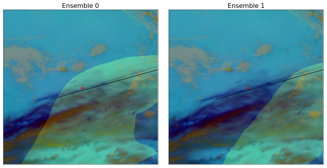
Figure 1 An example of the method used in this work. The red dot is the location of an in-situ measurement which shows ice supersaturation, and the yellow region denotes the locations where the given ensemble member predicts ice supersaturation at the time and altitude of the measurement. The satellite image is a false color image taken 30 min after the in-situ measurement, using the infrared bands as described in (Ng et al., 2023), with a detected contrail marked with the black line. Because our method applies a higher weight to “Ensemble 0”, the location of the contrail formation region it predicts better matches the observed contrail, and this leads to better agreement with the in-situ measurement.

For each in-situ measurement, we find all the flight waypoints within a threshold in distance, altitude difference and time difference. If the majority of those waypoints were found to match a contrail we label this in-situ measurement as observed = True, otherwise we label it observed=False. We then linearly interpolate the weather ensemble data to the location of the in-situ measurement.

We then compute the “contrail score” (S_hybrid), a unitless number between 0 and 1 where a higher score indicates a higher likelihood that a contrail formed, from this weather and observational data. This is similar to Hanst et al. (2025), who use a contrail score which is the fraction of ensemble members predicting persistent contrail formation conditions, here denoted S_{ensemble mean}. For our contrail score, we will combine the observations and ensemble weather forecasts using the following formula:

$$\begin{array}{}\text{(1)}& \begin{array}{rl}& S_{\mathrm{hybrid}}=\\ & \left\{\begin{array}{ll}\frac{\mathrm{TPR}\times S_{\text{ensemble mean}}}{\mathrm{TPR}\times S_{\text{ensemble mean}}+\mathrm{FPR}\times (\mathrm{1}-S_{\text{ensemble mean}})}& \mathrm{observed}=\mathrm{True}\\ \frac{(\mathrm{1}-\mathrm{TPR})\times S_{\text{ensemble mean}}}{(\mathrm{1}-\mathrm{TPR})\times S_{\text{ensemble mean}}+(\mathrm{1}-\mathrm{FPR})\times (\mathrm{1}-S_{\text{ensemble mean}})}& \mathrm{observed}=\mathrm{False}\end{array}\right.,\end{array}\end{array}$$

where $\mathrm{TPR}/\mathrm{FPR}$ are the true/false positive rate of the observation system. Equation (1) is just Bayes theorem where S_{ensemble mean} is “prior probability”, (the initial guess at the probability that a persistent contrail will form), and $\mathrm{TPR}/\mathrm{FPR}$ are the probabilities of observing a contrail on a flight which did/did not actually create a contrail. Another way to interpret the model scores is in the context of the weights in a weighted average over ensembles. The model score is the sum of the weights of all the ensemble members that predict a contrail. For S_{ensemble mean} this is just the fraction of ensembles predicting contrails, but for S_hybrid these ensembles get lower or higher weights depending on whether a contrail is observed.

2.2 Data

Numerical weather data comes from the European Centre for Medium-Range Weather Forecasts (ECMWF). We studied both the forecast (IFS) and reanalysis (ERA5) (Hersbach et al., 2020) product, and both nominal and ensemble products. The nominal and ERA5 ensemble data use the “model-level” weather products which have a vertical resolution of ≈10 hPa while for the IFS ensembles due to bandwidth constraints when downloading the data we use the “pressure-level” data which has a resolution of 25 hPa. Resolutions are 0.25° for the ERA5 nominal weather, 0.5° for the ERA5 ensemble weather, and 0.1° for the IFS weather. The ERA5 ensemble weather is at a time resolution of 3 h while all other products have a 1 h resolution. In order to compensate for the well-known dry bias (Gierens et al., 2020) of ECMWF high-altitude humidity data, we scale up the humidity field by dividing by 0.97 (Schumann, 2012; Jeßberger et al., 2013).

In-situ weather measurements are from the In-Service Aircraft for a Global Observing System (IAGOS; Boulanger et al., 2018 https://www.iagos.org/, last access: 30 January 2026). IAGOS uses instruments mounted on commercial aircraft to collect a variety of atmospheric data, we used the temperature and specific humidity measurements. The time and spatial resolution of IAGOS measurements is far greater than that of our numerical weather data. We therefore grouped the measurements into bins based on the altitude (rounded to the nearest flight level), time (rounded to the nearest hour), latitude and longitude (rounded to the nearest 0.25°) and randomly selected one measurement from each bin.

Contrail observations are obtained following the methods of Geraedts et al. (2024) and Sarna et al. (2025), summarized here. We first automatically detect contrails in GOES-ABI imagery (Ng et al., 2023). We then obtain flight waypoints from ADS-B data licensed from https://flightaware.com (last access: January 2026). We advect the waypoints using ERA5 wind data with a Runge Kutta 3D method, and additionally sediment downwards using the terminal velocity of an estimated ice crystal size average. Finally we compare the locations of the advected flights to the locations of the detected contrails. If these are close enough over multiple frames (details in Sarna et al., 2025) we say that the flight waypoints are observed to be matching a contrail. Note that the advection is uncertain because the wind data used is imperfect and contains errors of around 12.4 km h⁻¹ (Sonabend-W et al., 2026); the attribution algorithm accounts for this when it sets the tolerances of what flights can match an observed contrail.

The data used in this work was in the region shown in Fig. 2, covering the terrestrial Americas. We only have ADS-B data from terrestrial receivers so flight waypoints away from land are not included. The date range covered is 4 April to 31 December 2019 and 1 January to 31 December 2024. Our method has some tunable parameters, as defined below. We split our dataset by day of year and set aside every sixth day as the training set. The results in this work are evaluated on the remainder of the dataset. The complete dataset contains approximately 90 000 data points.

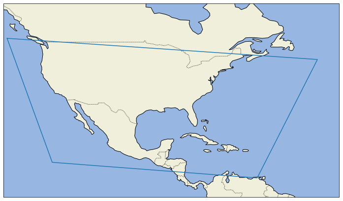
Figure 2 The region covered in this study is contained in the blue box.

Some of our results in this work come from simulating contrails using the pycontrails v0.60.3 (Shapiro et al., 2024) implementation of the CoCiP (Schumann, 2012) contrails model. CoCiP is a parameterized physics model of contrail evolution which includes formation, initial downdraft, advection and sedimentation, continually reassessing whether the contrail persists or sublimates. We configured CoCiP using the Poll-Schumann model of aircraft performance data (Poll and Schumann, 2021), and we adapted the humidity inputs to CoCiP using the “histogram matching” method, which recalibrates the forecast humidity to better match in-situ observations (Platt et al., 2024).

2.3 Metrics for comparing with in-situ measurements

We will use the above contrail score to predict whether the in-situ measurements will show persistent contrail formation conditions. We define “persistent contrail formation conditions” as the Schmidt-Appleman criterion (SAC) being satisfied and ice supersaturation (ISS), i.e. the relative humidity over ice (RHi) ≥100 %. The SAC requires aircraft information which is not in general defined for in-situ measurements, we used default values of 0.3 for overall efficiency and 1.25 for H₂O emissions index. In Sect. 3.1 we will also experiment with other contrail formation conditions.

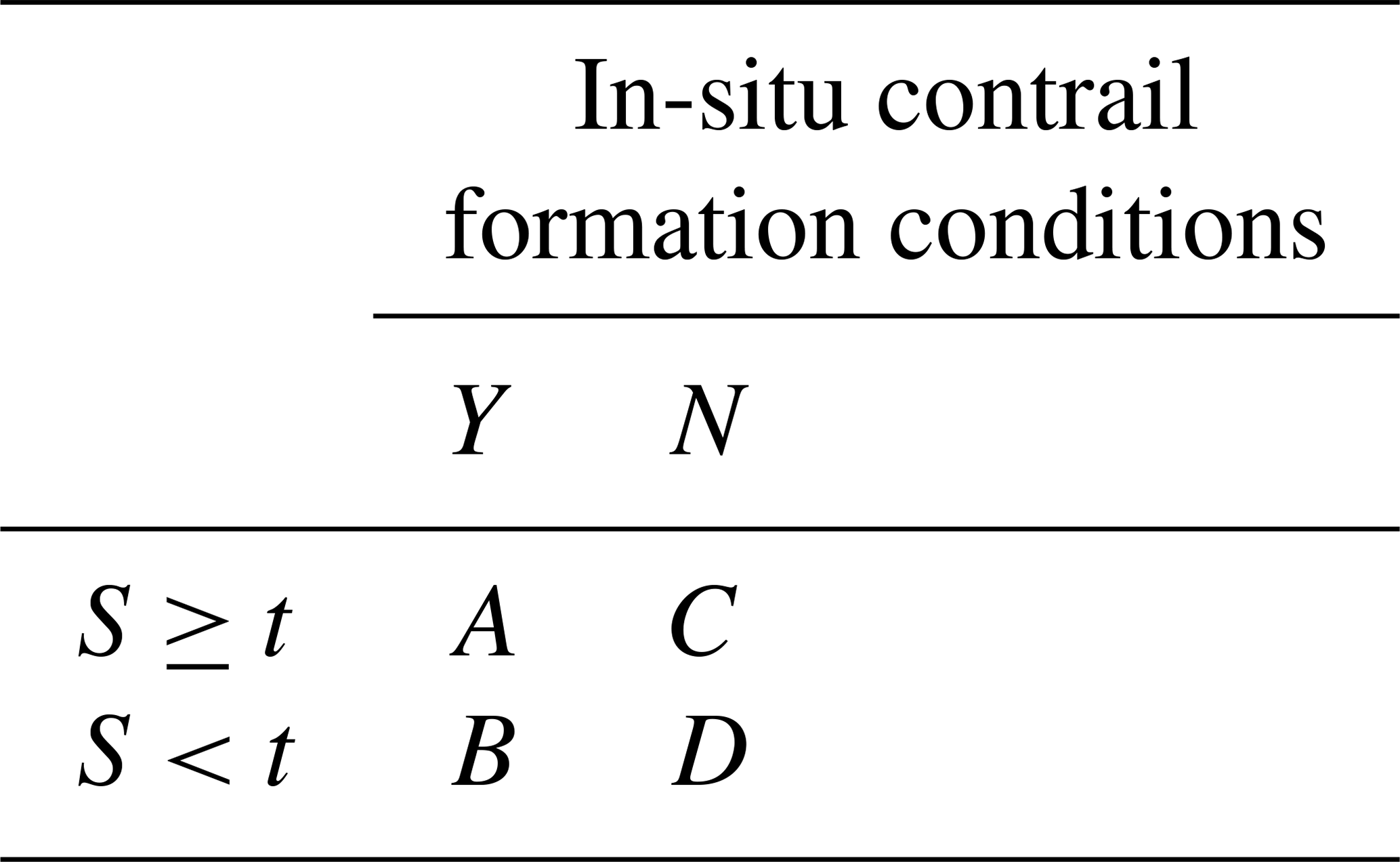
We assess the performance of different contrail verification systems by computing a contingency table like the one in Table 1. We then compute from the table “precision” $\equiv A/(A+B)$ and “true positive rate” (TPR) $\equiv A/(A+C)$. In the table S can be any contrail score, such as S_hybrid or S_{ensemble mean}. Since these contrail scores take continuous values we can create a curve on a precision/recall chart by varying the value of the threshold t. We will also consider the contrail score S_nominal which is simply whether the nominal weather predicts contrail formation conditions, and S_obs, the score based purely on observations. These scores are either 0 or 1 so t=1 is the only contingency table that we compute.

Table 1 Example of a contingency table used in this work. Here S is a contrail score and t is a threshold above which we say that the contrail score predicts persistent contrail formation conditions.

2.4 Defining distance thresholds

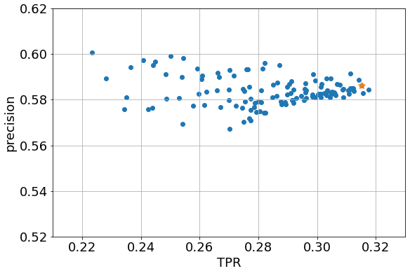
We say an in-situ measurement has observed contrails whenever nearby flights are observed making contrails. If there are multiple nearby points the observed value is set to true if any of the points have observed contrails. We now define what “nearby” means, in terms of thresholds in distance, altitude and time. To do this we do a grid search over these thresholds. The search covered 5–50 km in distance, 10–300 m in altitude and 120–3600 s in time. For each set of thresholds, we compute S_obs, the contrail score based solely on whether an in-situ point has observed contrails, on the training dataset defined in Sect. 2.2. Note that smaller distance thresholds naturally have a harder time finding nearby flight observations. The largest thresholds found 17 005 matching observations, we limited our results to thresholds that found at least 15 000. The results are shown in Fig. 3. From these results we chose a set of thresholds which give high TPR and precision. We choose the following thresholds:

$$\begin{array}{ll}{\displaystyle }\mathrm{distance}& {\displaystyle }=\mathrm{15}\mathrm{km}\\ {\displaystyle }\mathrm{altitude}& {\displaystyle }=\mathrm{20}\mathrm{m}\\ \text{(2)}& {\displaystyle }\mathrm{time}& {\displaystyle }=\mathrm{300}\mathrm{s}\end{array}$$

A sensitivity analysis with some other choices of distance parameters is given in Sect. 3.1.

Figure 3 Precision$/$TPR for S_obs for a number of different distance thresholds. The starred point is the one we chose, corresponding to the thresholds in Eq. (2).

2.5 Estimating performance of observation system

Equation (1) includes the true positive rate (TPR) and false positive rate (FPR) of our observation system. We estimate these parameters using synthetic data, using methods described in detail in (Sarna et al., 2025) and summarized here. In a contingency table like Table 1, $\mathrm{TPR}\equiv A/(A+B)$, $\mathrm{FPR}\equiv C/(C+D)$, but the contingency table compares to synthetic data rather than in-situ measurements. We start by simulating contrail evolution using CoCiP for all flights in a region covering most of North America, for 28 d spread out over the interval April 2019–April 2020. We use the simulated optical properties of these contrails to make synthetic contrail masks which are qualitatively similar to the masks produced by our contrail detector. Then we use our attribution system to attribute the flight paths to the synthetic contrails. In this simulated environment we know which flights actually made contrails, so we can assess how well the contrail attribution system worked. In Sarna et al. (2025) a fraction of flight waypoints were dropped to simulate aircraft without ADS-B transponders. This reduced TPR since those flights could never be attributed. In this work we do not drop these flights, which assumes the user of the contrail score has access to location data for all the flights they are interested in. Note that the CoCiP simulations used in SynthOpenContrails make no attempt include interactions between different contrails which may lead to an overestimation of contrail impacts in high contrail density areas (Rosenow and Luo, 2026). Also note that the synthetic data is generated using different wind data than that used during flight attributions, so measurements of the overall system performance include the effects of imperfect wind data.

To get the true/false positive rate, we need to define which contrails the observation system should be trying to find. We define this as all contrails with a total long-wave energy forcing $>\mathrm{5}\times {\mathrm{10}}^{\mathrm{13}}$ J. Such contrails are responsible for 96 % of the total warming in our synthetic dataset, so this is a reasonable group to target. With this definition we find

$$\begin{array}{}\text{(3)}& \mathrm{TPR}=\mathrm{33}\mathit{\%},\mathrm{FPR}=\mathrm{0.7}\mathit{\%}.\end{array}$$

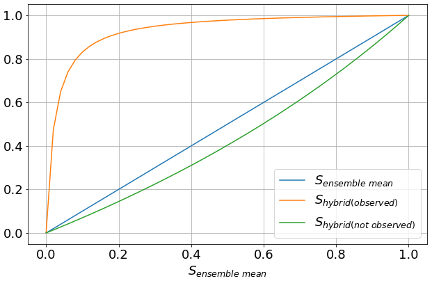
Figure 4 shows the results of putting these values into Eq. (1). Because FPR is small, a contrail observation is taken as strong evidence that a contrail is in fact formed. Therefore S_{hybrid(observed)} is much higher than S_{ensemble mean}. On the other hand TPR is not that close to one, so a lack of contrail observations is only weak evidence that no contrail is actually present. Therefore S_{hybrid(not observed)} is only slightly reduced compared to S_{ensemble mean}. The TPR number is per-contrail, but because more warming contrails are larger and longer-lived, they are more likely to be observed. The observation system captures 33 % of contrails but those contrails account for 42 % of the long-wave energy forcing.

Figure 4 Scores computed using Eqs. (1) and (3). We can see that observing a contrail leads to a large increase in score compared to S_{ensemble mean}, while not observing a contrail leads to a small decrease in score.

The $\mathrm{TPR}/\mathrm{FPR}$ values used here should be treated as estimates only. Their computation is based on the assumptions present in CoCiP, as well as the assumptions in Sarna et al. (2025) about how contrail properties translate into contrail detections. For example, in order to better match observed results Sarna et al. (2025) removes some simulated contrail detections in areas of high contrail density. This naturally lowers the TPR. But our simulations do not model contrail-contrail interactions, which means that they are likely overestimating the contrail impact in these regions (Rosenow and Luo, 2026). The TPR reported here assumes that our contrail simulations are correct, but the truth may be partway between the simulations and our synthetic observations. The metrics are also dependent on how the contrails detections at high contrail density are removed. Sarna et al. (2025) used a method which qualitatively matched real contrail detections but did not analyze if other methods could achieve as good or better agreement with real images. A sensitivity analysis to the TPR$/$FPR values is given in Sect. 3.2.

2.6 Estimating the energy forcing of contrails

In this section we define a contrail energy forcing estimate which takes into account both observations and ensemble weather. Energy forcing is the total radiative impact of the contrail. It is obtained by integrating the contrail radiative forcing over the width and length of the contrail, and over the contrail lifetime (Schumann et al., 2011). A reasonable way to estimate contrail energy forcing in the absence of observations is to simply simulate contrails using CoCiP for each member of the ensemble, and average the results. Since ensembles that don't predict contrail formation also predict zero forcing, this is equivalent to averaging the energy forcings of only the ensemble members that predicted contrail formation, and multiplying by S_{ensemble mean}. To generalize this we write

$$\begin{array}{}\text{(4)}& {\mathrm{EF}}_X=S_X{\mathrm{EF}}_{\mathrm{contrail}}.\end{array}$$

where S_X is any contrail score (S_{ensemble mean}, S_hybrid, etc) and EF_contrail is the mean warming over all ensemble members which predict a contrail.

3 Results

3.1 Including observations increases agreement with in-situ measurements

Figure 5 shows the precision and TPR for S_nominal, S_{ensemble mean} and S_hybrid, compared to the in-situ measurements, for the ERA5 and IFS weather products. S_hybrid has the best agreement with the in-situ measurements.

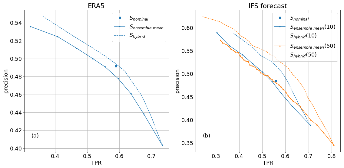
Figure 5 Precision$/$TPR plot for different contrail scores. We see that S_hybrid has the highest values, implying the best agreement with in-situ observations. This pattern is true for both (a) reanalysis and (b) forecast data. For the forecast data the (10) curves use 10 ensemble members while the (50) curves use 50.

We see that S_{ensemble mean} does not perform better than S_nominal, a surprising result which is different to that found by Hanst et al. (2025) (which uses a different numerical weather product). We expect that this is because the ensemble weather has a coarser spatiotemporal resolution than the nominal weather.

For the forecast product where 50 ensemble members are available, we see that S_hybrid performs better with more ensemble members. This is especially true at the high-TPR (TPR > 0.5) part of the curve, likely because more ensemble members increases the resolution of S_{ensemble mean}, making it better able to estimate the steep slope of S_{hybrid(observed)} in Fig. 4.

One might expect the ERA5 reanalysis weather to always agree better with in-situ measurements than the forecast, since the reanalysis has assimilated weather data up to the time of the reanalysis observation. This is true of S_nominal, but S_{ensemble mean} and S_hybrid are more mixed, with ERA5 performing better at the high recall parts of the curve while IFS performs better at high precision. However since the forecast and reanalysis weather have different resolutions we cannot clearly separate the effects of just changing from reanalysis to forecast data.

Computing the “hybrid” prediction requires satellite imagery, flight ADS-B data and weather data. The satellite imagery is available around 10 min after the image is taken, and the flight ADS-B data are available in near-real time. The good performance of the forecast weather in Fig. 5b means that in principle the results of the hybrid method could be made available almost immediately after the flight time, allowing immediate feedback for aircraft operators on whether contrails were formed.

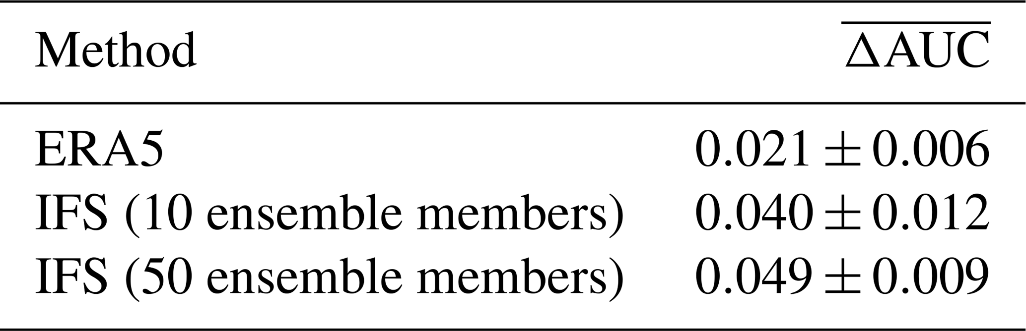
We can summarize Fig. 5 by computing the area under the curves (AUC) of the different forecasts. We define $\stackrel{\mathrm{‾}}{\mathrm{\Delta }\mathrm{AUC}}$ as the difference in the AUC between two curves, computed only in the TPR range where the curve is present, and divided by the size of the TPR region. Another interpretation of $\stackrel{\mathrm{‾}}{\mathrm{\Delta }\mathrm{AUC}}$ is the average precision difference between the curves. In Table 2 we show $\stackrel{\mathrm{‾}}{\mathrm{\Delta }\mathrm{AUC}}$ for a few different cases. Error bars are 2 standard deviations obtained by bootstrap sampling the dataset 1000 times. Since points at similar locations and times may be correlated, during the bootstrapping we kept all data points on the same day together rather than sampling each data point individually.

Table 2 $\stackrel{\mathrm{‾}}{\mathrm{\Delta }\mathrm{AUC}}$ for a few different cases.

We also experimented using only ice supersaturation (ISS) rather than the combination of the Schmidt-Appleman criterion and ice supersaturation (SAC + ISS) as the definition of “persistent contrail formation conditions”. The improvement of S_hybrid over S_{ensemble mean} is smaller for ISS-only than for SAC + ISS. ($\stackrel{\mathrm{‾}}{\mathrm{\Delta }\mathrm{AUC}}=\mathrm{0.008}\pm \mathrm{0.010}$ for ISS-only).

This is because in cases where ISS predicts a persistent contrail but SAC is not satisfied, no contrail actually forms. When our observations (correctly) observe no contrail, if we defined “persistent contrail formation conditions” as ISS-only, then this correct observation hurts the performance of S_hybrid in our metrics. The improved benefit for using observations when evaluating SAC + ISS is therefore simply because SAC + ISS is better at predicting the formation of persistent contrails than ISS alone.

3.2 Insensitivity of results to hybrid parameters

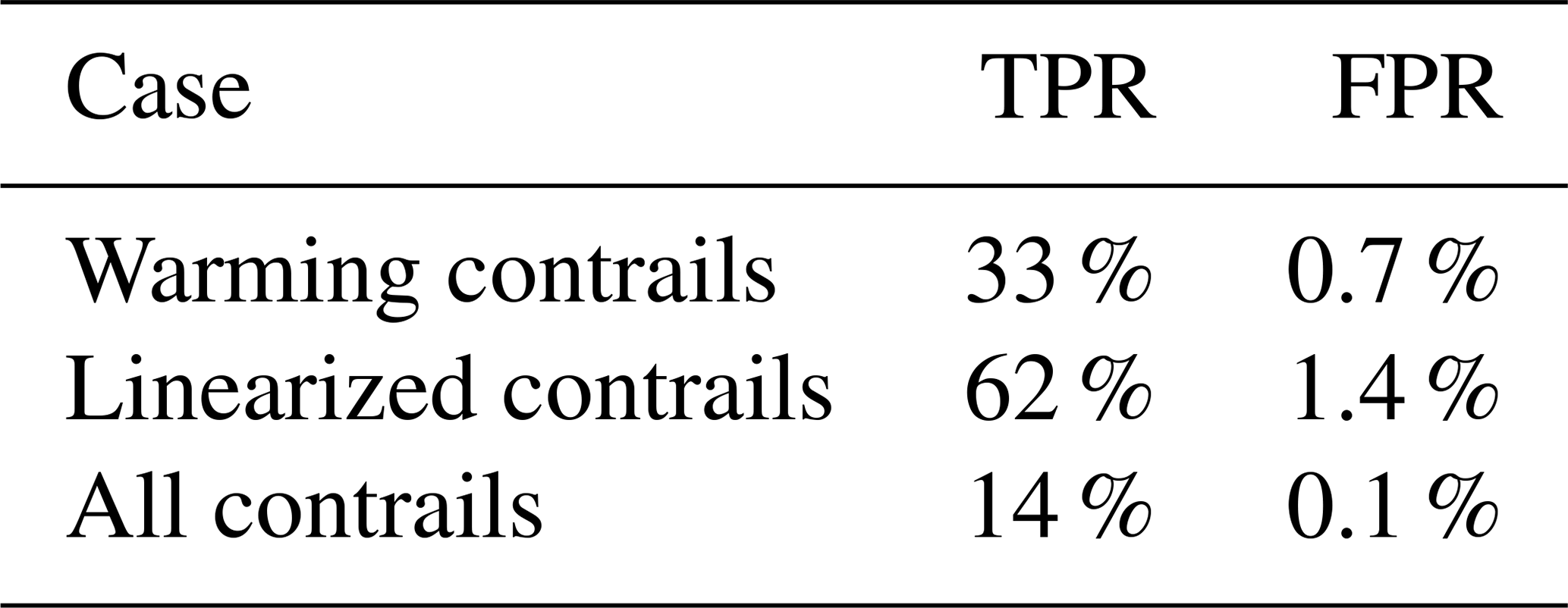
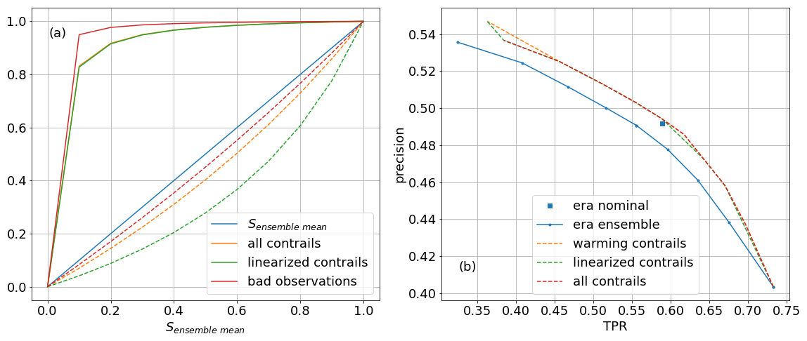
We now perform a sensitivity analysis of our results to the TPR$/$FPR values in Eq. (1). The other values tested are shown in Table 3. The “Warming contrails” case is defined in Eq. (3) and used in the other results in this work. The “Linearized contrails” case is comparing the matched contrails from the SynthOpenContrails dataset only to the synthetic contrails that survived the rasterization and linearization process in Sarna et al. (2025). The biggest difference compared to the “Warming contrails” case is that SynthOpenContrails intentionally removes contrail detections in high contrail density areas to match the results on real images. The “Warming contrails” case assumes that these high contrail density detections are missing in real images because the contrail detector cannot resolve them, while the “Linearized contrails” case assumes that if CoCiP correctly simulated contrail-contrail interactions these contrails would not have formed. The “All contrails” case compares the observation system to all the contrails predicted by CoCiP with nonzero energy forcing. Figure 6a shows how S_hybrid changes in the different cases. All cases have low TPR, so in all cases the effect of observing a contrail is to dramatically increase S_hybrid relative to S_{ensemble mean}. Relative to the “warming contrails” case the linearized (all) contrails case has higher (lower) TPR, which leads to larger (smaller) decrease in S_hybrid when a contrail is not observed. In particular the very small TPR in the “all contrails” case means that a non-observation barely changes the contrail score. Figure 6b shows the impact on S_hybrid's agreement with in-situ measurements. We see that the agreement is not very sensitive to the choice of TPR$/$FPR, and outperforms S_{ensemble mean} in all cases.

Table 3 Alternate TPR$/$FPR values (replacing those in Eq. 3 evaluated in Fig. 6).

Figure 6 (a) Same as Fig. 4 but including the different choices of TPR$/$FPR outlined in Table 3. For each case solid lines show S_{hybrid(observed)} and dashed lines show S_{hybrid(not observed)}. (b) Same as Fig. 5a, but the dashed lines show different S_hybrid for the different cases in Table 3.

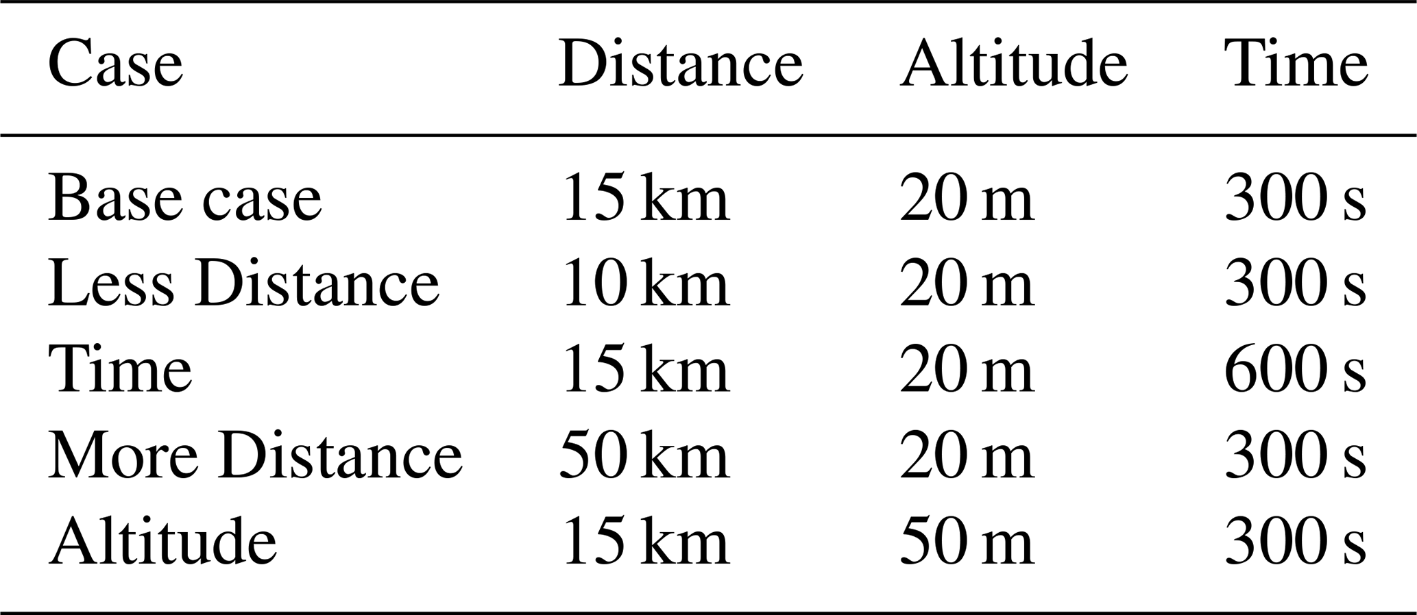
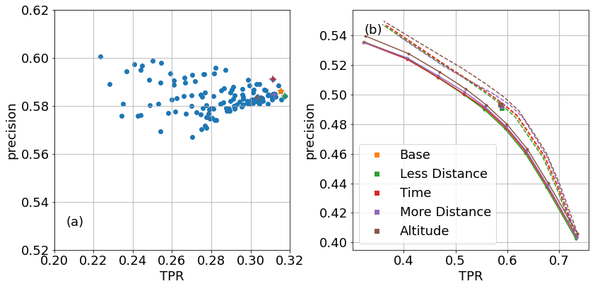
We also perform a sensitivity analysis of our results to the thresholds in Eq. (2). The other values tested are shown in Table 4. The base case is the one used elsewhere in this work, in this analysis we include points with increased time, distance and altitude threshold which still perform relatively well in TPR and precision. Figure 7a shows the TPR and precision of these cases on our training dataset. Figure 7b shows the effect of the different thresholds on the various contrail scores. Note that different thresholds include different points in the evaluation dataset, so each of the cases is evaluated on a slightly different dataset. In all cases the pattern of $S_{\mathrm{nominal}}⪅S_{\text{ensemble mean}}<S_{\mathrm{hybrid}}$ is present. Figure 7a shows the largest sensitivity to altitude, potentially because the supersaturated layers that drive contrail formation are often vertically thin.

Table 4 Alternate thresholds evaluated in Fig. 7.

Figure 7 (a) Same as Fig. 3 but including the different thresholds in Table 4. The orange star shows the base case while the crosses show the other cases. (b) Same as Fig. 5a, but covering the different cases shown in Table 4.

3.3 Comparison of aggregate energy forcing values

We can also compare the warming values from Eq. (4). We chose one day per month in the span June 2024–May 2025 and computed EF_{ensemble mean} and EF_hybrid for all the flights in Fig. 2. The resulting dataset (which is different from the dataset used in the rest of this work) contains ≈430 000 flights. We report energy forcing per meter (EF^pm) by summing the energy forcings and flight distances over all flights in the dataset:

$$\begin{array}{}\text{(5)}& {\mathrm{EF}}_X^{\mathrm{pm}}={\displaystyle \frac{{\sum }_i\mathrm{EF}\left(i\right)}{{\sum }_{i}L\left(i\right)}}.\end{array}$$

We find

$$\begin{array}{}\text{(6)}& {\displaystyle }{\mathrm{EF}}_{\text{ensemble mean}}^{\mathrm{pm}}& {\displaystyle }=\mathrm{15.50}\pm \mathrm{0.12}\mathrm{MJ}{\mathrm{m}}^{-\mathrm{1}}\text{(7)}& {\displaystyle }{\mathrm{EF}}_{\mathrm{hybrid}}^{\mathrm{pm}}& {\displaystyle }=\mathrm{15.55}\pm \mathrm{0.12}\mathrm{MJ}{\mathrm{m}}^{-\mathrm{1}},\end{array}$$

where the error bars are obtained by taking 2 standard deviations of 100 bootstrap samples. The fact that these values agree is partially by design as we chose the TPR$/$FPR values in Eq. (3) relative to synthetic CoCiP data. If we instead use the “Linearized contrails” TPR$/$FPR values from Table 3 then ${\mathrm{EF}}_{\mathrm{hybrid}}^{\mathrm{pm}}$ is 13 % lower than the ${\mathrm{EF}}_{\text{ensemble mean}}^{\mathrm{pm}}$, because (at least according to CoCiP) the contrails which form but do not create linear features in the SynthOpenContrails dataset do contribute some warming which those TPR$/$FPR values would not capture. If we use the “All contrails” TPR$/$FPR values we find that ${\mathrm{EF}}_{\mathrm{hybrid}}^{\mathrm{pm}}$ is 6 % higher than ${\mathrm{EF}}_{\text{ensemble mean}}^{\mathrm{pm}}$, because in that case we are penalizing the TPR value to account for contrails which have only very small forcing. Figure 8 shows the aggregate forcing as a function of local hour. Both EF_{ensemble mean} and EF_hybrid show expected pattern of warming contrails at night and small forcing during the day.

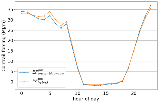
Figure 8 Energy forcing as a function of local time of day, for both ${\mathrm{EF}}_{\text{ensemble mean}}^{\mathrm{pm}}$ and ${\mathrm{EF}}_{\mathrm{hybrid}}^{\mathrm{pm}}$. We see that both have similar values and exhibit the expected diurnal pattern of warming at night and ambiguous results during the day.

4 Discussion and Future Work

In this work we defined a “contrail score” S_hybrid which combines ensemble weather and contrail observations, and saw that it compared better to in-situ measurements than scores based entirely on weather data. We used this to define a method of estimating contrail warming which weights ensemble members by their agreement with observations, and showed that though the hybrid method is more correct on a per-contrail basis, it produces similar aggregate values to methods using only weather data.

In this work we used the aircraft-based IAGOS system as a source of in-situ measurements, but the method does not require the measurements to be on aircraft and future work could compare to other in-situ measurements such as from radiosondes.

This work shows that contrail observations can improve estimates of meteorological quantities related to contrails. We tested this approach using an 10-ensemble-member reanalysis product with low resolution and a 50-ensemble-member forecast product with higher resolution. We found that more ensemble members, and higher resolution improves performance, suggesting that the best possible estimates of whether a flight made a contrail could be obtained by a reanalysis product with higher resolution and more ensemble members. Another improvement might be to increase the number of ensemble members well beyond 50, for example by using an AI weather model (Kurth et al., 2023).

The approach taken in this work is a very basic method of combining observations and weather, and the fact that it leads to an improvement suggests that more sophisticated approaches, such as assimilating contrail observations directly into a weather model, may be worth pursuing. One could also try imposing spatial/temporal consistency on these ensemble weights, as opposed to this work where the weights are chosen independently for each measurement. Better agreement with in-situ measurements would be one way to assess the impact of such improvements, but there are others. It would be desirable if a future approach produced a more physically consistent set of weather fields. This would allow one to estimate warming by running a physical model once on the new weather data, which would be computationally cheaper than the approach in this work of running the physical model on each ensemble member and taking the weighted average of the results. The improvements in this work only apply to points near a flight path. This is not a problem for contrail avoidance applications since by definition we care most about points near flight paths, but extending the distance the improvements apply over could allow contrail observations to improve weather for non-contrail applications.

Another interesting direction could be to generalize the techniques in this work to other weather data. For example, one could try to improve wind data by weighting weather ensembles based on whether they agree with the observed motion of persistent contrails.

The contrail score and warming estimates produced in this work used CoCiP to determine the TPR$/$FPR values in Eq. (1) and to estimate warming. CoCiP is not the only method of estimating the evolution of contrails and other methods can give different contrail properties in case studies (Akhtar Martínez et al., 2025; Kärcher and Corcos, 2025). Further research is needed to determine if these differences yield significant changes in agreement with in-situ measurements or aggregate contrail forcing. The methods used in this work can be straightforwardly adapted to use a different contrail model if desired.

In this work we showed that contrail observations can help to predict in-situ measurements of SAC and ISSR. In-situ measurements of SAC and ISSR are a proxy of what we really want to observe, which is persistent contrail formation. These measurements must be a pretty good proxy, (otherwise contrail observations would not help to predict them), but they are likely not a perfect proxy due to both noise in the in-situ measurements and physical phenomena (e.g. wake-vortex interactions, advection, sedimentation) which are not modeled. In Sect. 3.1 we saw how more accurate proxies of persistent contrail formation led observing a larger benefit of using observations. This is because in the results in this work every time the proxy incorrectly predicts a contrail and observations (correctly) do not observe one (and vice-versa), we count that as a mistake by the observations. Therefore we expect that the results in this work are understating the benefits of incorporating observations, a hypothesis which could be tested by comparing with improved “ground-truth” datasets, such as those being developed using ground cameras (Jarry et al., 2026).

For the purposes of determining whether an aircraft made a contrail, both weather models and geostationary imagery have limitations (Agarwal et al., 2022; Gierens et al., 1999; Driver et al., 2025; Euchenhofer et al., 2025). This work shows that despite their limitations, both approaches have complementary information and therefore taking them together leads to the best estimates of whether an aircraft made a persistent contrail.